Ray tracing in relativistic stars
From geometry
to observation
How spacetime curvature decides the image, the spectrum and the light curve that an X-ray telescope receives from a neutron star.
Outline
Four parts, one path
I
The star inside
What holds a neutron star up: the TOV equation, the equation of state and the mass–radius curve.
II
Relativistic ray tracing
Null geodesics in Schwarzschild: light bending, redshift and time delays — and how to follow the rays backwards, from the telescope to the surface.
III
Pulsars and neutron stars
The laboratories: pulsars and magnetars, hot spots, rotation, atmospheres — and what NICER has already measured.
IV
Recent results
My work: magnetar light curves, a massive low-field magnetar, accretion columns — and tests of alternative theories of gravity.
The premise
Everything we know arrives as photons
Compact stars are natural laboratories of strong-field gravity — but we know them only through the photons that left them and crossed a curved spacetime.
The direct problem
Given the star and the metric, predict what is observed. That is ray tracing.
The inverse problem
Given what is observed, infer mass, radius, spot geometry and magnetic field.
The test
If the metric is not Schwarzschild, the light curves change: observation tests gravity.
I
Part one
The star
inside
Before following the light, the source: what holds more than a solar mass within 12 km — the pressure of the densest matter we know, against the gravity of general relativity.
Anatomy · a TOV solution with the SLy equation of state
From the crust to the unknown core
- Atmosphere and ocean: centimetres to metres of H, He or C — where the light of Part II comes from.
- Outer crust: a lattice of ever more neutron-rich nuclei in a sea of electrons, up to 4×10¹¹ g/cm³, when neutrons start to drip out of the nuclei.
- Inner crust: nuclei and free, superfluid neutrons; at the bottom, “nuclear pasta”. Up to ~ρ₀/2.
- Outer core: neutrons, with some protons, electrons and muons, up to ~2ρ₀.
- Inner core: up to ~6ρ₀. Hyperons? Free quarks? The equation of state decides.
ρ₀ = 2.7×10¹⁴ g/cm³ is the density inside an atomic nucleus. TOV profile with SLy (Douchin & Haensel 2001, in the piecewise polytropes of Read et al. 2009).
Tolman · Oppenheimer & Volkoff · 1939
Hydrostatic equilibrium in general relativity
pressure has inertia
Pressure is energy, and energy resists acceleration like mass. At the centre of this star: ×1.15
pressure gravitates
Pressure is also a source of gravity and adds to the mass. At the centre: ×1.46
space curves
Radial distances stretch, and the factor grows outwards. At the surface: ×1.55
More pressure, more gravity: squeezing harder is not enough, and a maximum mass appears — which Newton does not have.
The equation of state
How hard matter resists being squeezed
- The equation of state gives the pressure as a function of density, P(ρ): what the TOV needs to close.
- Up to ~ρ₀ laboratory nuclear physics constrains the curve; above, each model extrapolates: two- and three-nucleon forces (WFF1, APR4), Skyrme (SLy), relativistic Brueckner–Hartree–Fock (ENG, MPA1), relativistic mean field (MS1; H4, with hyperons).
- Stiff — more pressure at the same density — gives a bigger, heavier star; soft, a smaller, lighter one.
- Limits: sound cannot outrun light, and 2 M☉ pulsars rule out the softest.
cs²/c² = ΓP/(ε + P). The dot marks the centre of the maximum-mass star; beyond it, the curve is faded. The jumps come from the polytrope fit, which changes Γ at 1014.7 and 1015 g/cm³; near the centre of the heaviest stars some fits exceed c.
Tolman–Oppenheimer–Volkoff · equation of state
From nuclear physics to the M–R curve
Each equation of state P(ε) gives a mass–radius curve and a maximum mass. Measuring the mass and radius of the same star picks between them.
The lines of constant compactness look ahead to Part II: below R = 1.76 RS the whole surface is in view; at 1.5 RS lies the photon sphere.
Piecewise polytropes of Read, Lackey, Owen & Friedman (2009); constraints (68%): NICER — Riley et al. 2019, 2021; Miller et al. 2019; Choudhury et al. 2024; PSR J0348+0432 (Antoniadis et al. 2013); GW170817 (Abbott et al. 2018).
II
Part two
Relativistic
ray tracing
Near a mass, light does not travel in a straight line: it follows the null geodesics of the metric. Ray tracing means following those geodesics backwards — from the telescope to the source.
25 November 1915
Einstein and his field equations
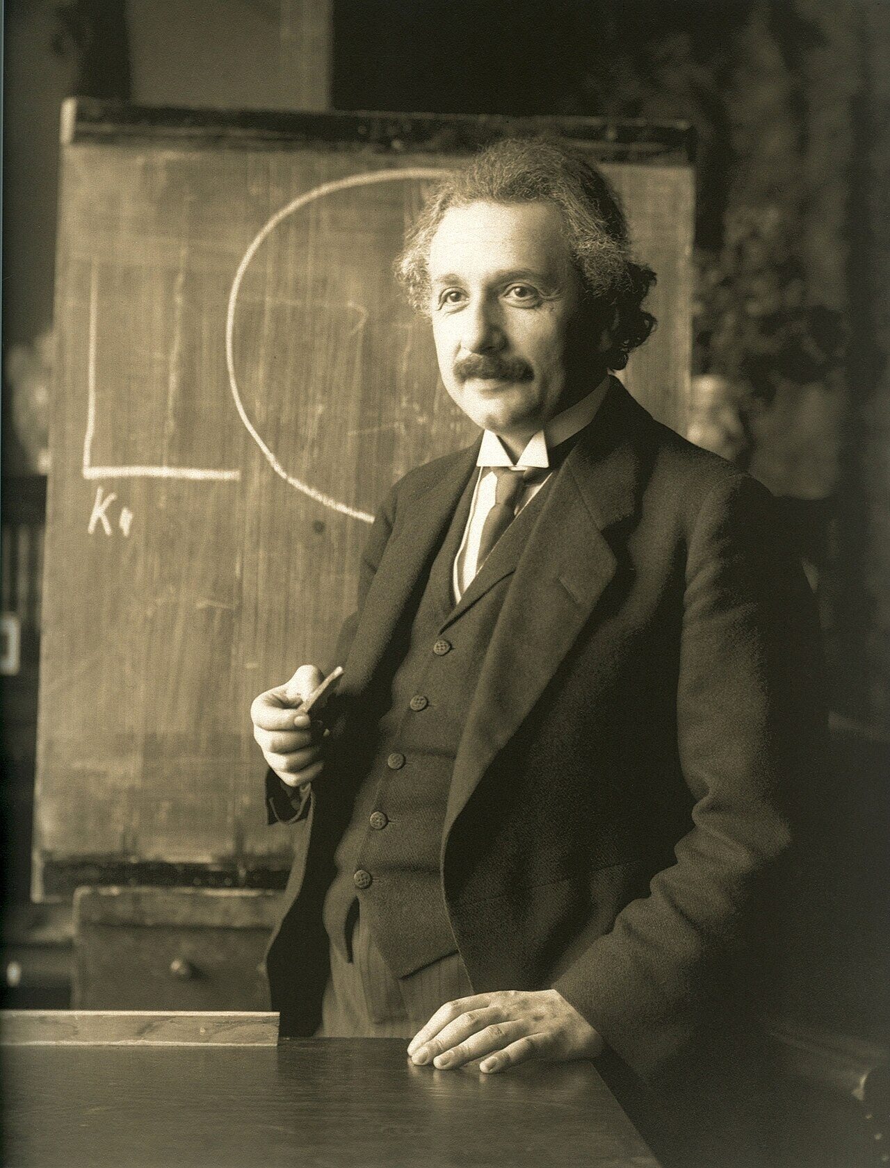
F. Schmutzer · public domain“Spacetime tells matter how to move; matter tells spacetime how to curve.”
The classical tests
Sobral, 1919: light bends
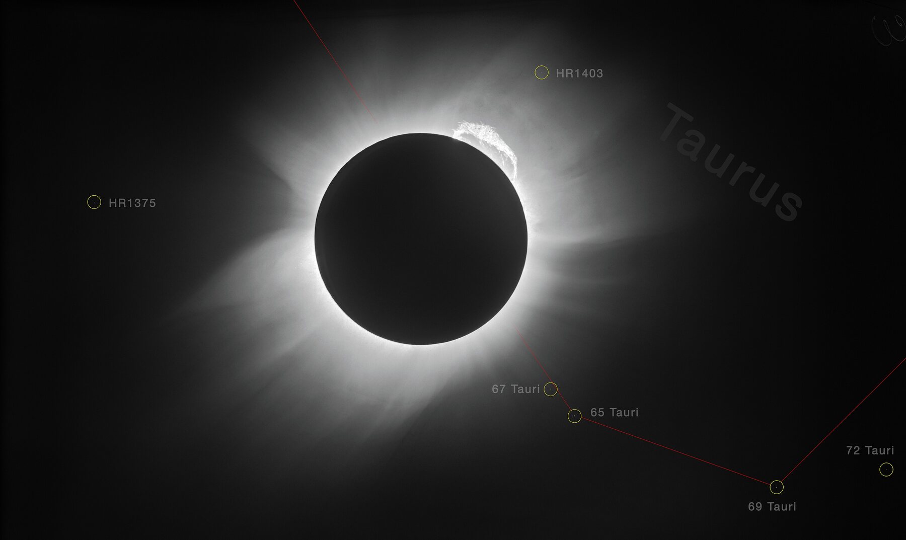
ESO / Landessternwarte Heidelberg-Königstuhl / Dyson, Eddington & Davidson · CC BY 4.0| effect | GR predicts |
|---|---|
| perihelion of Mercury (1915) | 43″ / century |
| light grazing the Sun (1919) | 1.75″ |
| redshift, Pound–Rebka (1959) | 2.5×10⁻¹⁵ over 22.5 m |
| Shapiro delay (1964) | ~200 μs |
| GPS clocks | +38 μs / day |
Sobral expedition (Ceará, Brazil): 1.98 ± 0.12″. Príncipe: 1.61 ± 0.30″. The sky over north-eastern Brazil confirmed Einstein.
Sobral, 29 May 1919 · the measurement
Two plates, the same sky
Night: the Hyades photographed in July, before dawn, with the same telescope — the Sun far away.
Eclipse: the same field on 29 May, with the Moon covering the Sun. Every star moves away from the Sun, radially.
On the whole plate nothing moves: 1″ is a tenth of a pixel. In the loupes, at true scale, as under the micrometer, the star jumps by a fraction of its own width — and the centre of a blob can be measured far better than its width.
Einstein’s calculation · November 1915
Where the 1.75″ comes from
1859 – 1915 · the perihelion of Mercury
Mercury’s orbit does not close
| perihelion advance | per century |
|---|---|
| observed (relative to the stars) | 574″ |
| other planets, by Newton | 531″ |
| unexplained remainder | 43″ |
Le Verrier found the remainder in 1859 and proposed a hidden planet, Vulcan. It was never found. Einstein got the 43″ with no adjustable parameter.
“For a few days, I was beside myself with joyous excitement.”
December 1915 · Russian front
Schwarzschild and the first exact solution
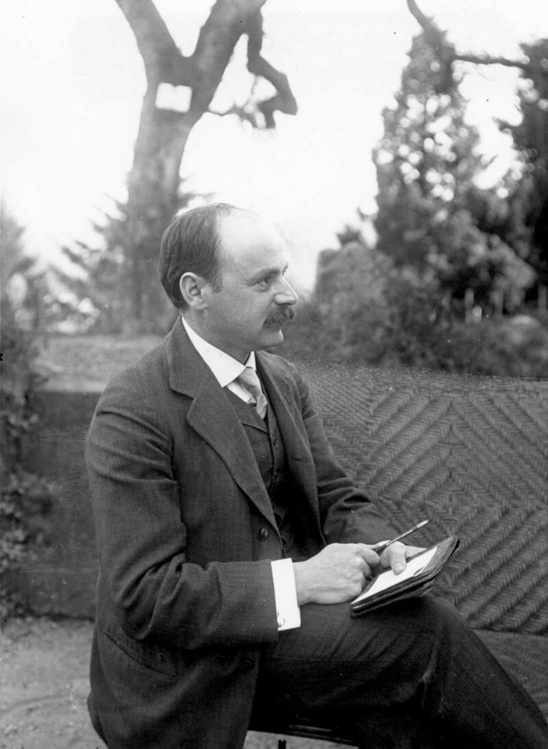
1 rs
event horizon
1.5 rs
photon sphere
3 rs
ISCO: last stable orbit
2.95 km
rs of the Sun (Earth: 8.9 mm)
He wrote to Einstein on 22 December 1915 while serving as an artillery officer. He died in May 1916.
What we need from the metric
Curvature does three things to a photon
1 · It bends the path
The photon follows a null geodesic. Near the surface of a neutron star the bending is tens of degrees: we see more than half of the star.
2 · It changes the energy
A photon emitted at r with local energy E reaches infinity with
3 · It delays
Different paths take different times (Shapiro delay): photons from each point of the star arrive tens of microseconds apart.
Ray tracing puts all three into a single calculation, pixel by pixel, for each instant of the rotation.
In a neutron star, R ≈ 2.5–3 RS: none of the three effects is a small correction.
And all three depend only on the metric outside the star — which is why a light curve carries information about gravity.
Null geodesics in Schwarzschild
Two constants and a potential
The metric depends on neither t nor φ: energy and angular momentum are conserved.
For light only the ratio matters, the impact parameter b = L/E:
The maximum of V lies at r = 1.5 RS: the photon sphere. Below bc = (3√3/2) RS the ray comes from the horizon — or from the star.
Schwarzschild geodesics
How light bends
- b > 3√3 GM/c² ≈ 2.6 RS: the light is deflected and escapes.
- b = 2.6 RS: unstable orbit on the photon sphere, r = 1.5 RS.
- b < 2.6 RS: captured.
The term on the right is the General Relativity correction. Without it, light would travel in a straight line.
Event Horizon Telescope · 2019 and 2022
The shadows
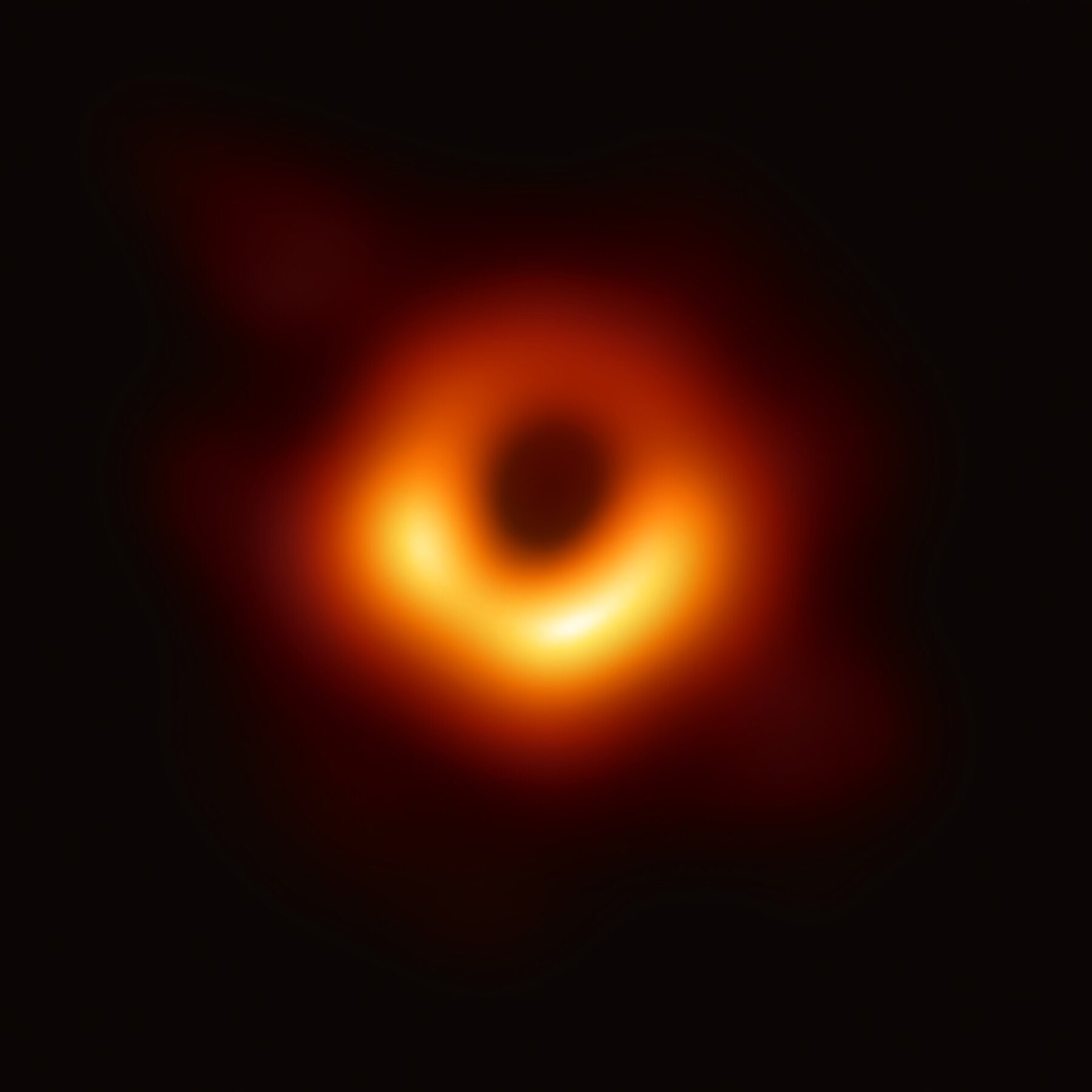
M87* · 2019 · 6.5 billion M☉ · 55 million light-yearsEHT Collaboration · CC BY 4.0
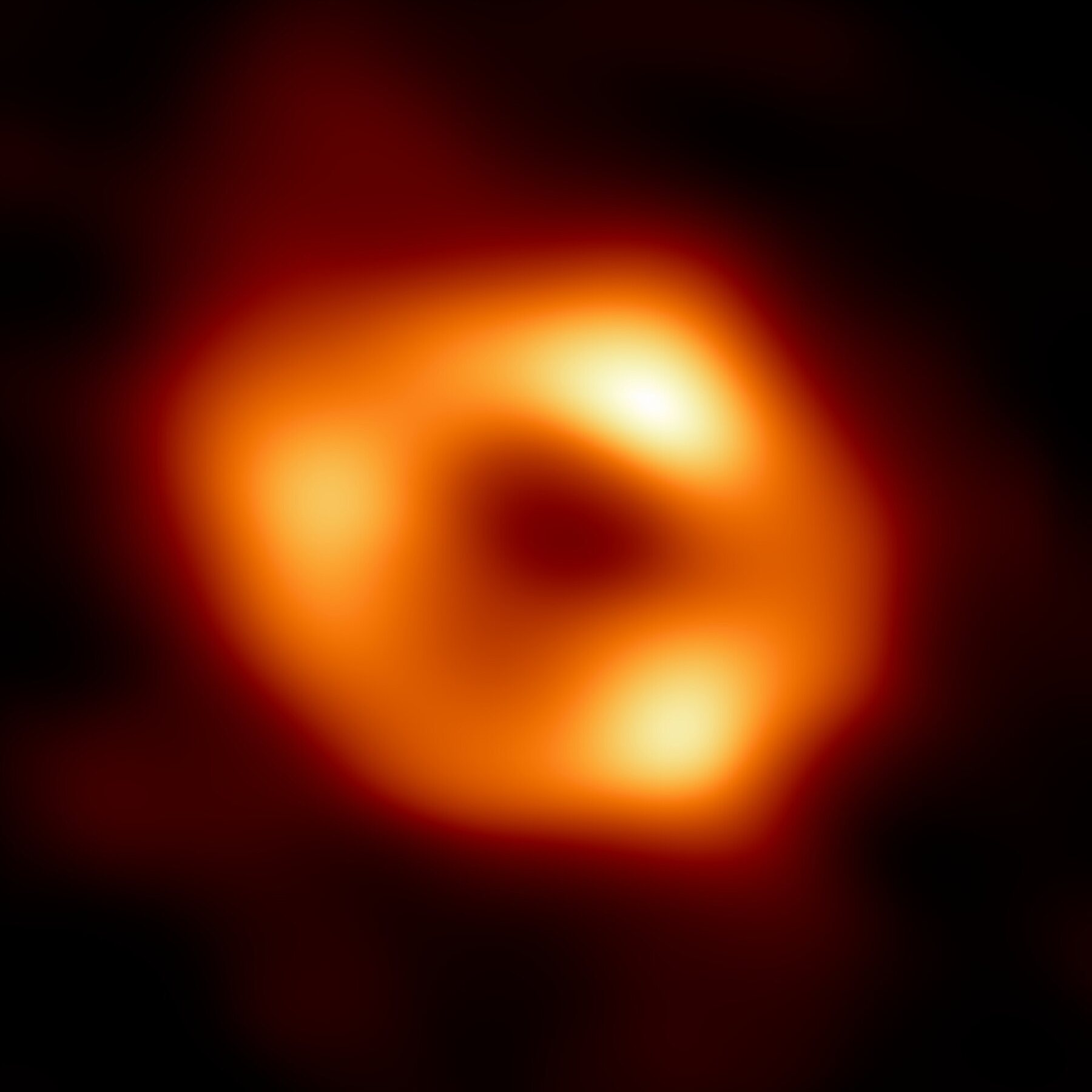
Sgr A* · 2022 · 4.3 million M☉ · 27,000 light-yearsEHT Collaboration · CC BY 4.0The ring is ~5 RS across: it is the photon sphere, at 1.5 RS, seen through the lens of the black hole itself — shadow diameter = 2√27 GM/c² ≈ 5.2 RS.
Compactness
Where GR stops being a correction
Surface compared with infinity: z = (1 − rs/R)−1/2 − 1, g = (GM/R²)(1 − rs/R)−1/2 · deflection from the exact orbit integral (weak field: 2rs/R) · ISCO, photon sphere and horizon: a 1.4 M☉ star of that size · the objects advance on their own until the first click.
The angle that matters
From the surface to infinity: ψ(α)
A photon leaves the surface at an angle α to the normal. By the time it reaches the observer, it has turned through ψ around the centre:
Without gravity, ψ = α and the limb is at 90°. With gravity, the limb moves further round: we see behind the star. The approximation is excellent down to R ≈ 3 RS and fails precisely where the secondary image appears.
The naive idea: from the star to the camera
Many rays, hardly any pixels
- Every point of the surface emits in every direction; each ray is followed along its geodesic, outwards.
- Only those that pass through the camera aperture become pixels: here, 2 in every 10,000.
- Completing this image would take ~10⁸ rays: hours of computing.
- With a real telescope, 1 m² at 1 kpc, 1 photon in every 10⁴⁰ arrives.
3D count: uniform point on the surface, isotropic outward direction, exact geodesic to the camera, at 13 RS. Only a sample is drawn, in the plane; the rays that enter the camera are all shown.
The method: from the camera to the star
One pixel, one ray
- The rays leave the camera, one per pixel: the path of light travelled backwards. The direction of the pixel gives the impact parameter b.
- The geodesic is integrated until the ray escapes to the sky or hits the surface at some point, at an angle α.
- The pixel takes the colour of the point the light left from — corrected for redshift and for the emission angle.
- Every ray computed becomes a pixel: 3,136 rays, 3,136 pixels, against the 10⁸ of the previous slide.
With spherical symmetry, ψ depends only on b: one table ψ(b), computed once, serves every pixel. Each ray is rotated into the plane of the drawing.
What a compact star looks like
We see behind the star
On the left, the star as it would look without gravity; on the right, ray-traced. The grid is the same; gravity bends the light around the star and reveals the far hemisphere.
- The image is larger: apparent radius R/√(1 − RS/R).
- For R < 1.76 RS the whole surface is visible — the far pole becomes a ring.
- Below 1.5 RS the star would lie inside the photon sphere.
1959 · Pound & Rebka · Jefferson tower, Harvard
Light loses energy as it climbs
14.4 keV γ rays from ⁵⁷Fe (Mössbauer effect). Pound & Rebka, PRL 4, 337 (1960): ~10%; Pound & Snider, Phys. Rev. 140, B788 (1965): ~1%. Every 12 s source and absorber swap places, as in the experiment.
Liouville · what reaches the telescope
The spectrum that climbs out of the well
Along a ray, Iν/ν³ is conserved. With g = √(1 − RS/R):
A black body stays a black body, only cooler. The luminosity seen from afar is L∞ = g² L.
A spectral line of known energy E0 arrives at g E0: measuring the line means measuring the compactness.
Part II in summary
The ray tracing recipe
- Choose the exterior metric: Schwarzschild; Hartle–Thorne or Kerr with rotation; a different one for a different theory of gravity.
- Build the table ψ(b) and the delay Δt(b) by integrating the null geodesics once.
- For each pixel (or each surface element): b → emitting point, angle α, redshift g, delay.
- Intensity: Iobs = g³ I(E/g, α′), with the atmosphere’s beaming and the Doppler shift from rotation.
- Add up: image, flux — and, phase by phase, the light curve and the phase-resolved spectrum.
Exact or approximate?
- Exact integral (or elliptic integrals): always valid, secondary images included.
- Beloborodov (2002) and Poutanen & Beloborodov (2006): closed formulae for ψ and for the delay, excellent for R ≳ 3 RS.
- Oblate Schwarzschild (Morsink et al. 2007): a star flattened by rotation, for millisecond pulsars.
This is the engine behind NICER’s mass and radius measurements — and behind the results of Part IV.
III
Part three
Pulsars and
neutron stars
The laboratories: more compact than anything short of a black hole, spinning, magnetised — and with their surface visible in X-rays.
Neutron stars in numbers
A solar mass in a city
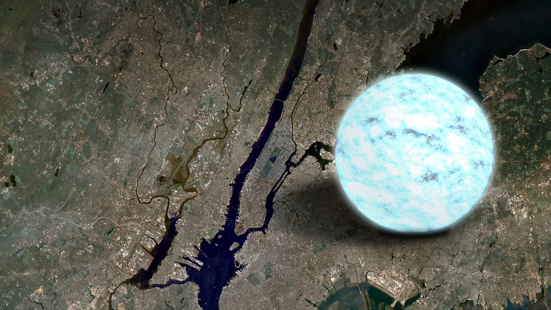
NASA's Goddard Space Flight Center · public domain1.1–2.1 M☉
measured masses
11–13 km
radius (NICER, gravitational waves)
2–3 RS
compactness: the regime of Part II
10⁸–10¹⁵ G
surface magnetic field
Central density a few times that of the atomic nucleus, ~10¹⁵ g/cm³. Spin periods from 1.4 ms to tens of seconds.
Surface gravity is ~10¹¹ times the Earth’s; the escape velocity, 0.5 to 0.7 c.
Cambridge · 28 November 1967
The first pulsar: “LGM-1”

Roger W Haworth · CC BY-SA 2.0

W. T. Sullivan III / NRAO/AUI · CC BY 4.0
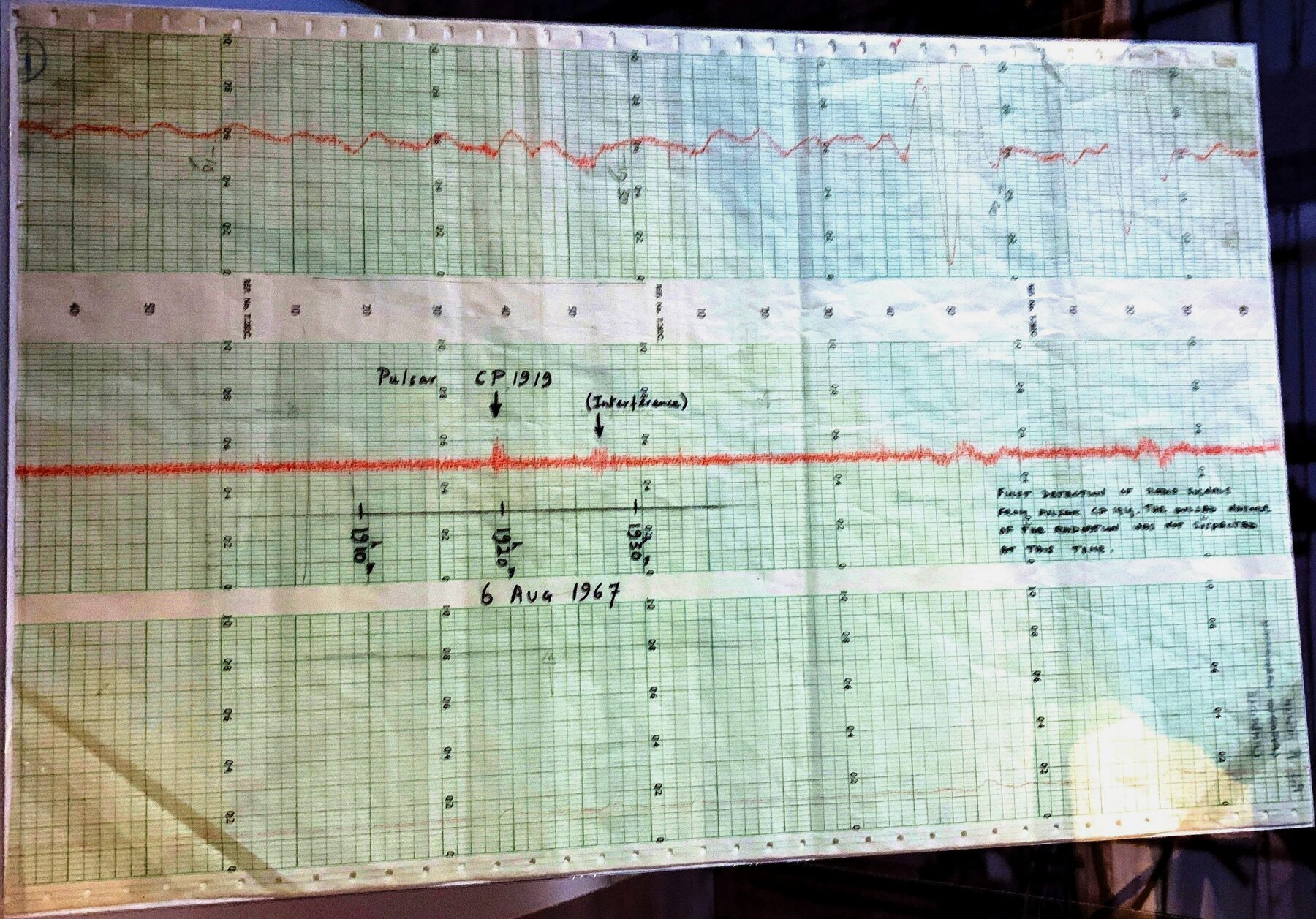
Bill Thompson · CC BY-SA 4.0Bell noticed a bit of “scruff” that kept coming back on the radio telescope’s paper chart: pulses every 1.337 s, as regular as clockwork. Nickname: LGM-1, for Little Green Men. It was a spinning neutron star.
Pulsar theory
What is measured, and what is inferred
| observable | expression |
|---|---|
| period | P |
| characteristic age | tc = P/2Ṗ |
| magnetic field | B = (3Ic³PṖ/8π²R⁶)1/2 |
| rotational energy lost | Ėrot = −4π²IṖ/P³ |
Canonical neutron star
M = 1.4 M☉ · R = 10 km · I = 10⁴⁵ g cm²
B = 3.2×10¹⁹ (PṖ)1/2 G
|Ėrot| = 3.9×10⁴⁶ Ṗ/P³ erg/s
Only P and Ṗ are measured. The rest comes from assuming a spinning magnetic dipole — the straight lines in the diagram.
Transient activity
A magnetar, spinning
| event | energy |
|---|---|
| short bursts (~0.1 s) | 10³⁹ – 10⁴¹ erg |
| outbursts (months) | 10⁴¹ – 10⁴³ erg |
| giant flares | 10⁴⁴ – 10⁴⁶ erg |
The field lines, anchored in the crust, get twisted over time. When the crust can no longer take the stress, it cracks — a starquake — and the magnetic energy comes out all at once.
Giant flares in the Galaxy and the Magellanic Clouds: 1979, 1998 and 2004.
The surface in X-rays
Why hot spots appear
Millisecond pulsars
Particles accelerated in the magnetosphere flow back and heat the polar caps to ~10⁶ K. They are NICER’s targets.
Magnetars
Field decay and the currents along twisted field lines heat regions of the crust — which change after each outburst.
Isolated cooling stars
The magnetic field makes heat conduction anisotropic: poles hotter than the equator (the “Magnificent Seven”).
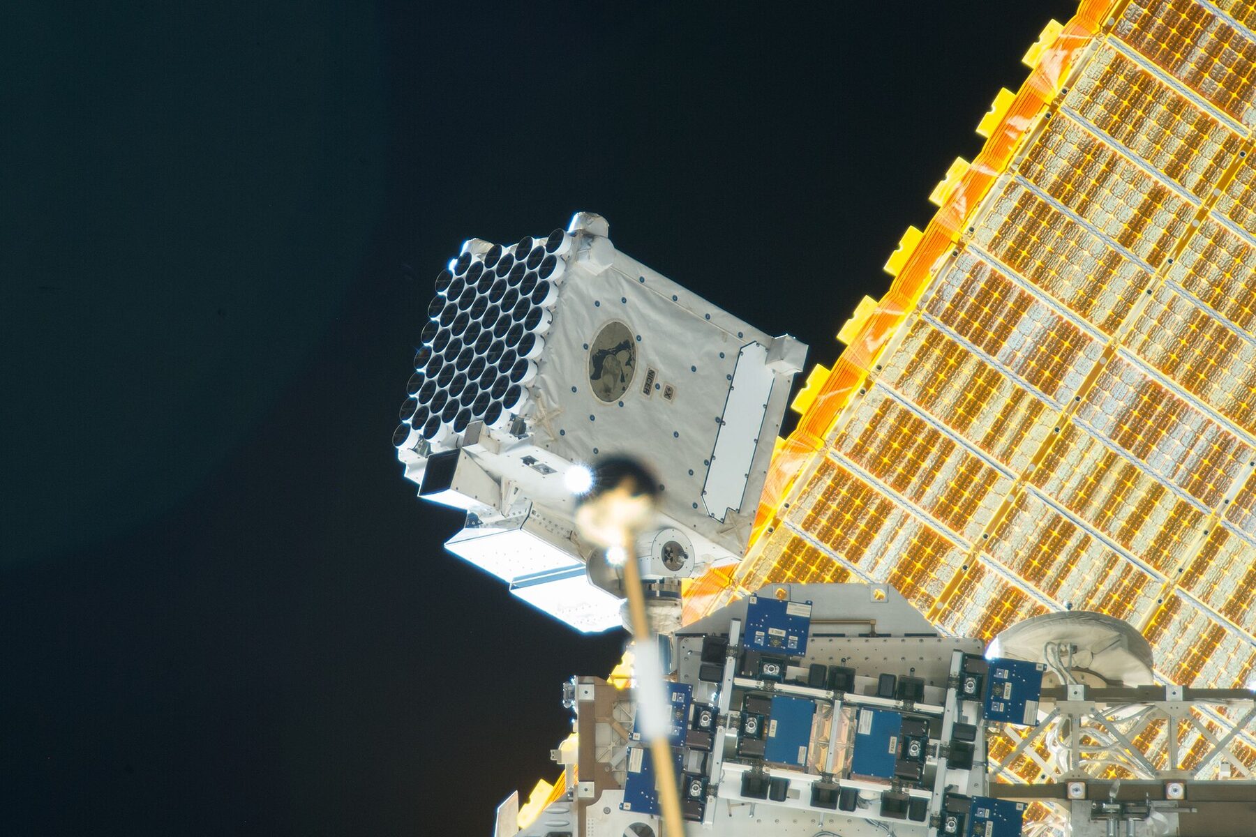
NASA · public domain
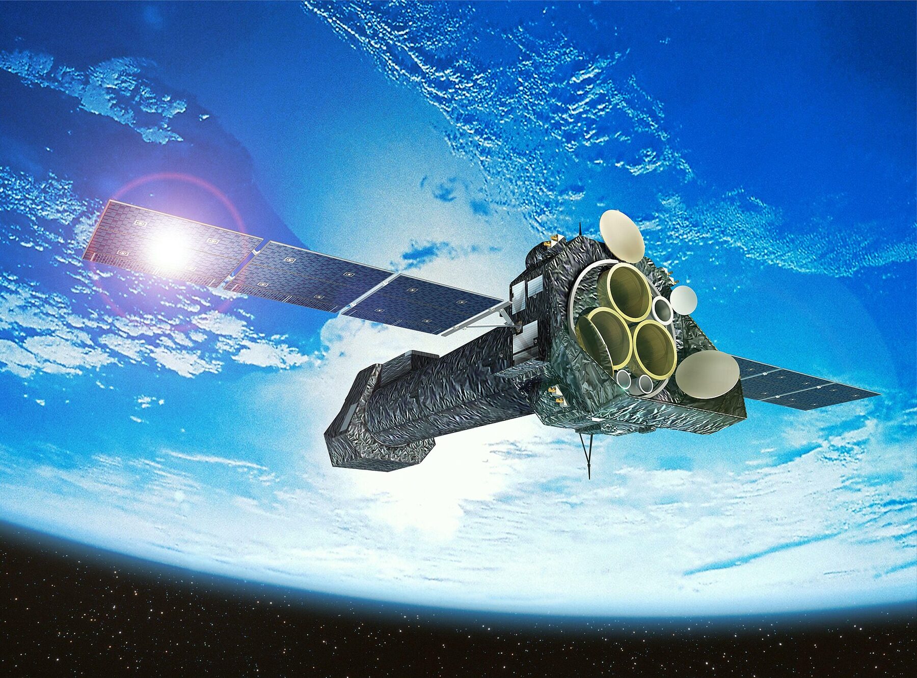
ESA/XMM-Newton · CC BY-SA 3.0 IGO
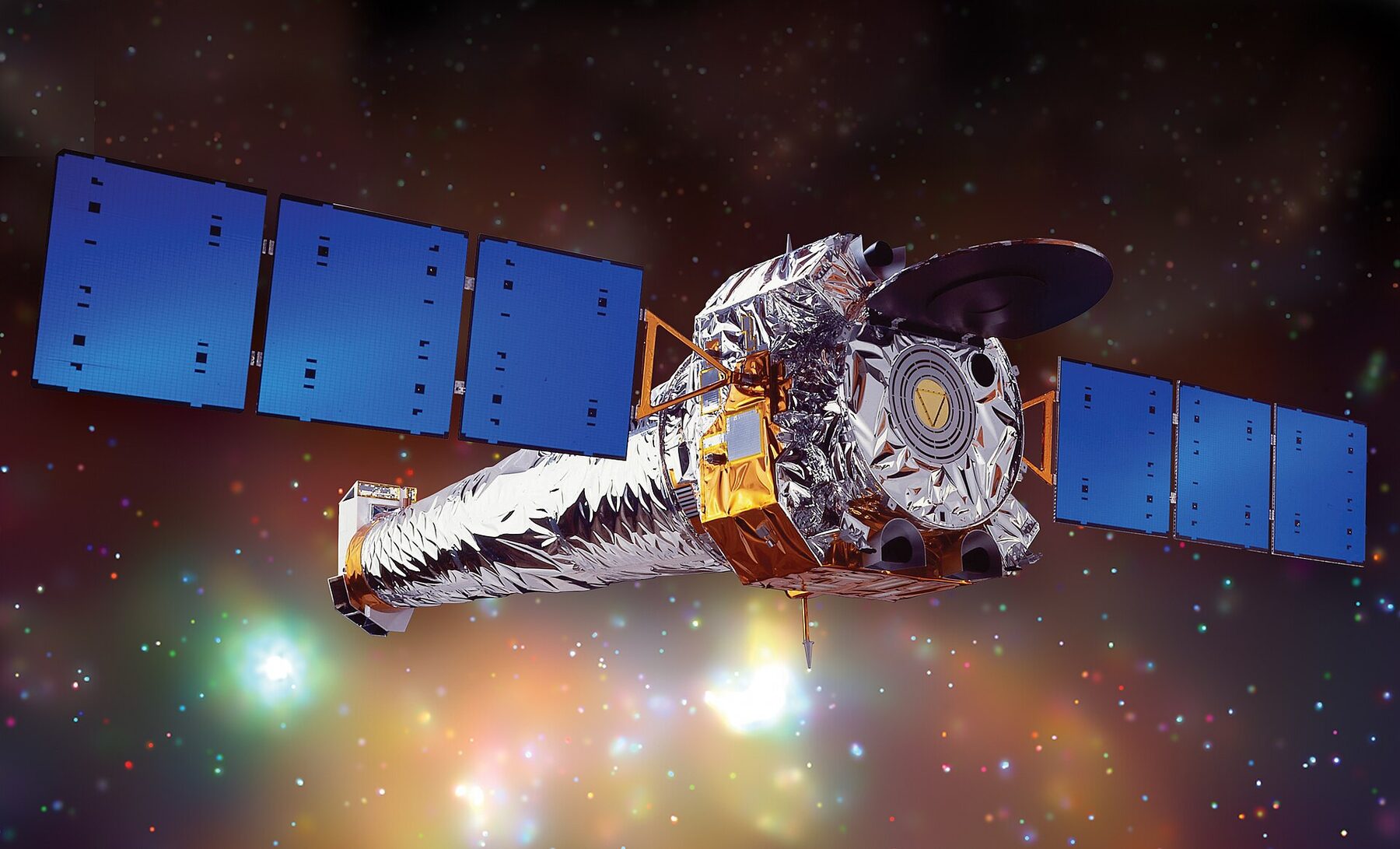
NASA/CXC/NGST · public domainRay tracing a hot spot
One spot, one light curve
Two spots · Beloborodov’s classes
Antipodal, or not
Rotation and atmosphere
Doppler, aberration, delays and beaming
- Doppler: the surface moves at up to 0.1–0.2 c; the approaching side is brighter (bolometric flux ∝ δ⁵).
- Aberration: the emission angle changes in the frame of the surface.
- Delays: tens of μs between points on the star — fractions of the period at hundreds of Hz.
- Beaming: an atmosphere does not emit equally in all directions; the profile depends on it.
Together they make the pulse asymmetric and create harmonics — and the asymmetry measures R separately from M.
NICER · pulse-profile modelling
Mass and radius from the pulse shape
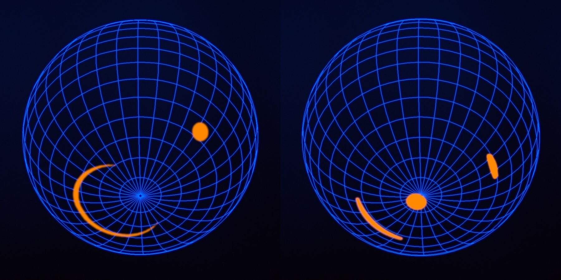
NASA/GSFC · public domain| pulsar | mass (M☉) | radius (km) |
|---|---|---|
| PSR J0030+0451 · Riley+ 2019 | 1.34+0.15−0.16 | 12.7+1.1−1.2 |
| PSR J0030+0451 · Miller+ 2019 | 1.44+0.15−0.14 | 13.0+1.2−1.1 |
| PSR J0740+6620 · Riley+ 2021 | 2.07+0.07−0.07 | 12.4+1.3−1.0 |
| PSR J0437−4715 · Choudhury+ 2024 | 1.42 ± 0.04 | 11.4+1.0−0.6 |
NICER time-stamps each photon to ~100 ns. Folding millions of photons at the period gives the pulse profile; ray tracing, with M, R, the geometry and the spots left free, fits that profile by Bayesian inference.
J0030’s spots came out non-antipodal and elongated: the field is not a centred dipole.
IV
Part four
Recent
results
Ray tracing applied to real data — magnetars, a massive magnetar, accretion columns — and the same tool used to test gravity beyond Einstein.
2017 – 2026
Light curves as an instrument
2017
A&A 599, A87: rotation-powered SGRs and AXPs, with realistic neutron stars
2020
ApJ 889, 165: SGR J1745−2900 and a multipolar field, from the light curve
2023
Galaxies 11, 18: pulse profiles of accretion columns
2024
JHEAp 42, 52: 3XMM J1852+0033, a massive low-field magnetar
2024
EPJC 84, 1337: light curves as a test of scalar-tensor gravity
2024
PRD 110, 103014: stratified rotation and the moment of inertia
2025
PRD 112, 083010: quark stars and the QCD equation of state
2026
arXiv:2607.09836: compact stars in a high-tension braneworld
2026
JHEAp (submitted): the column of 1A 0535+262 through its NuSTAR spectrum
The common thread: reading in the light of a compact star its mass, its radius, its field — and the gravity that curves it.
de Lima, Coelho, Pereira, Rodrigues & Rueda · ApJ 889, 165 (2020)
SGR J1745−2900: more than two spots
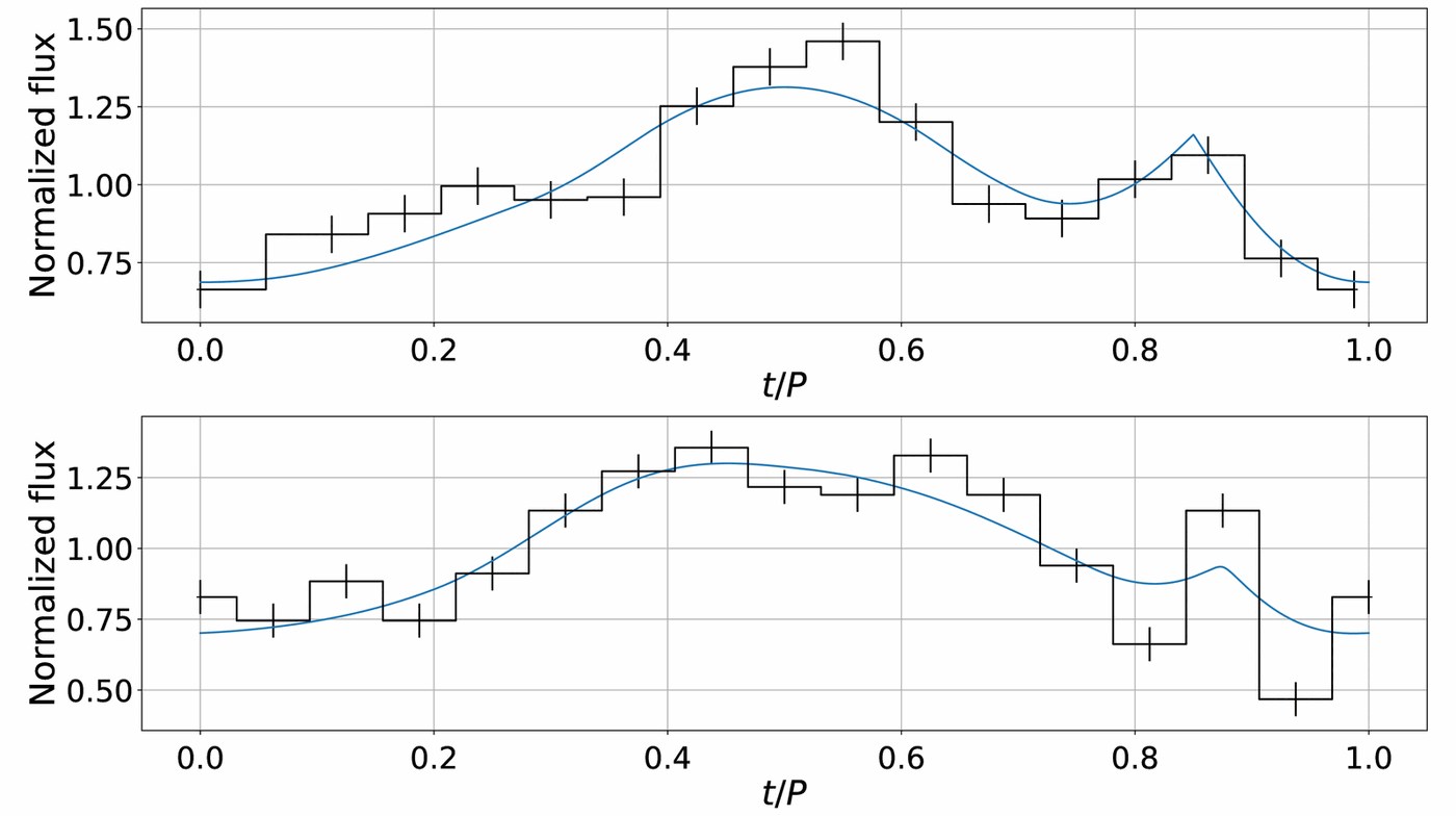
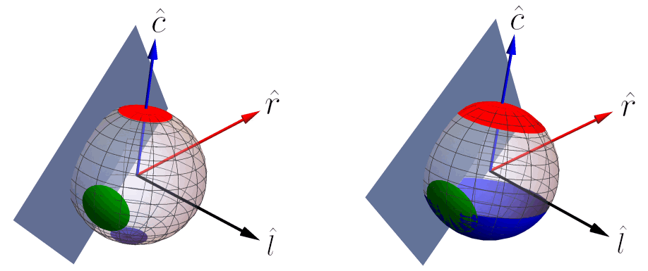
- The magnetar 0.1 pc from Sgr A*; 3.5 years of Chandra data.
- Model: M, R, up to three spots of any size and position, Schwarzschild light bending; fitted with a genetic algorithm.
- Two or three spots describe the data; with three, they are large (16–67°).
- A field with non-trivial poloidal and toroidal structure — the same message NICER gave for J0030.
1.4 ± 0.1
M☉
10.9 ± 1.5
km
de Lima et al. · JHEAp 42, 52 (2024) · 1/2
3XMM J1852+0033: ray tracing and inference
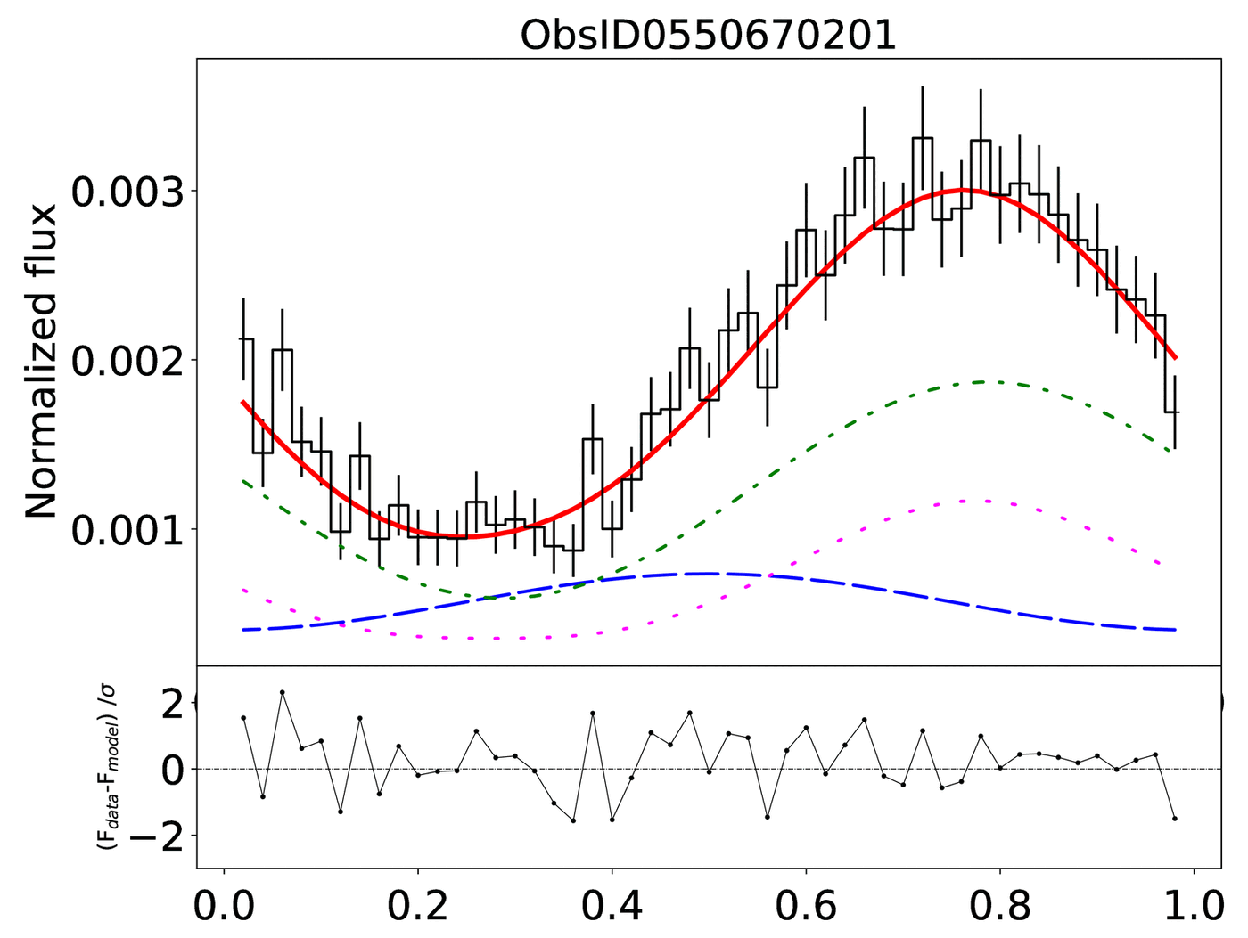
- A transient magnetar near the remnant Kes 79, P = 11.56 s; until then there were only upper limits on the field.
- Five XMM-Newton epochs over three weeks in 2008.
- Ray tracing in Schwarzschild with circular spots of any size (Turolla & Nobili 2013) and magnetised atmospheres (NSMAX: H, C, O), with anisotropic emission.
- Bayesian inference (MCMC): mass, radius, field and spot positions shared by all epochs; size and temperature free to vary.
- Tested by injection and recovery of simulated data.
Best model
Three small spots, two in the southern hemisphere, and a carbon atmosphere: χ²/dof = 1.22, well ahead of two spots or of hydrogen.
de Lima et al. · JHEAp 42, 52 (2024) · 2/2
A massive, low-field magnetar
2.09+0.16−0.09 M☉
mass (1σ): among the highest ever estimated
12.0 ± 1.4 km
radius (2σ)
~8×10¹¹ G
surface field: log B = 11.89+0.19−0.93, below the critical value
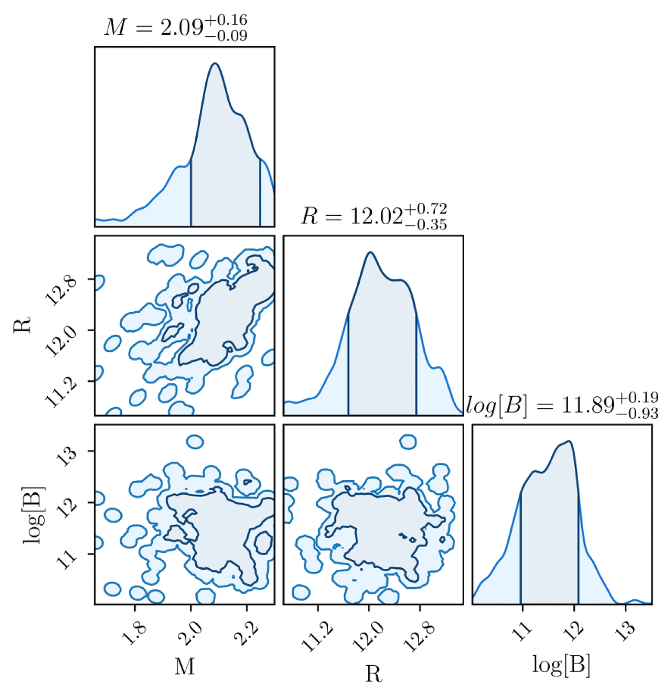
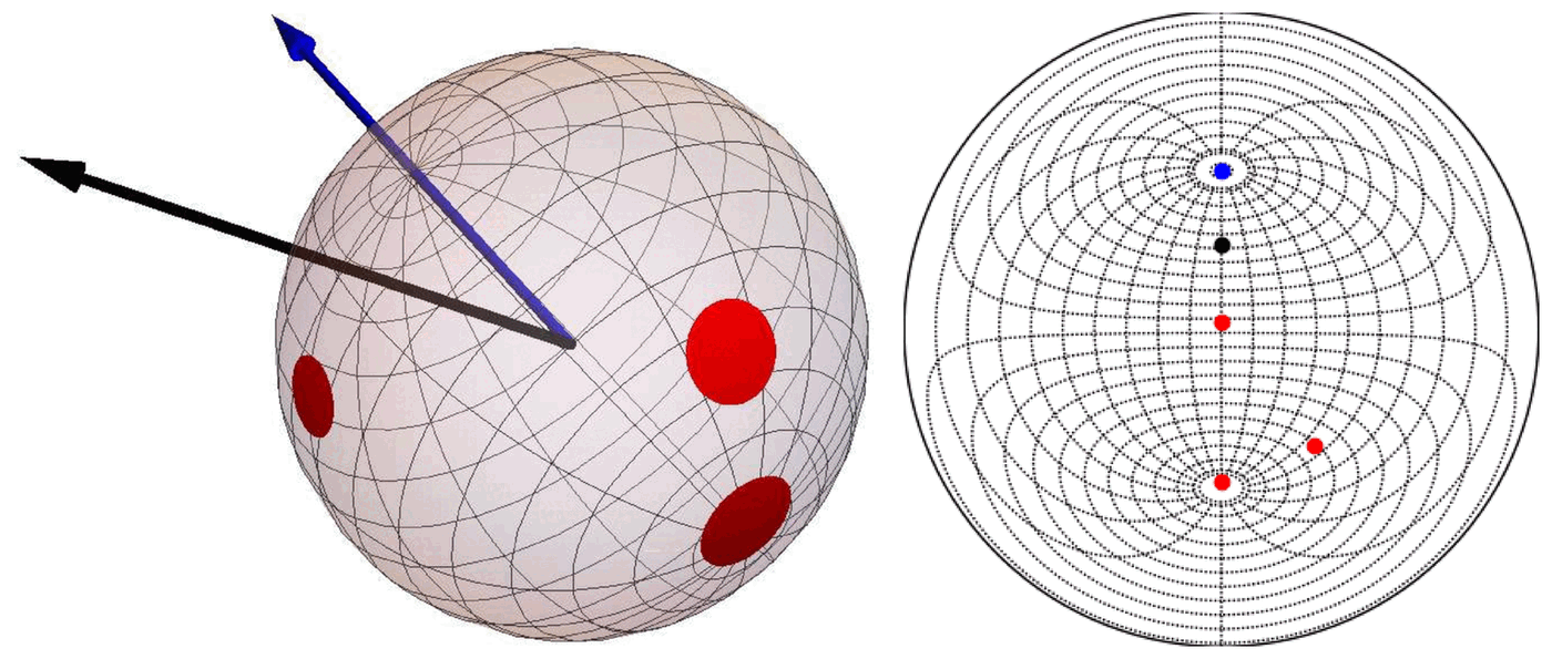
Interpretation: accretion of supernova material buried the field, which is now re-emerging; the carbon atmosphere would come from diffusive nuclear burning of H/He.
Compactness GM/Rc² ≈ 0.26: favours equations of state of intermediate stiffness.
Silva, de Lima, Coelho, Stecchini, de Liz & de Araujo · Galaxies 11, 18 (2023)
When the light comes from a column
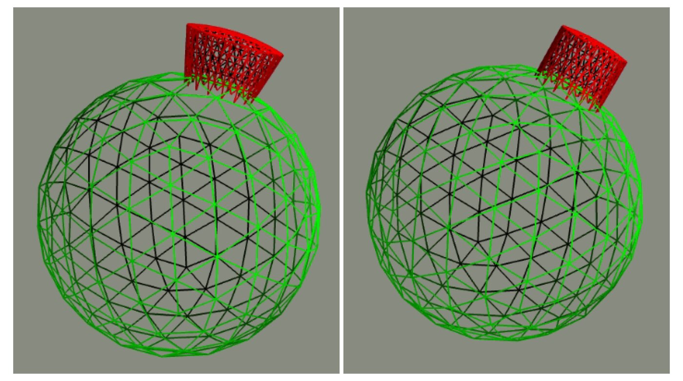
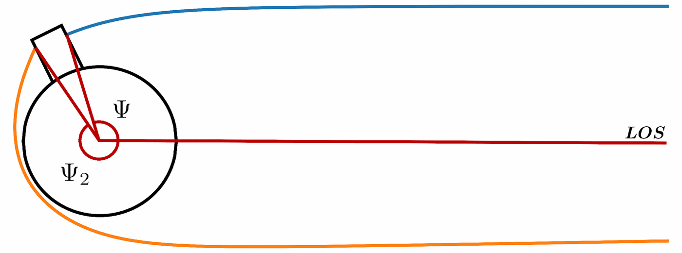
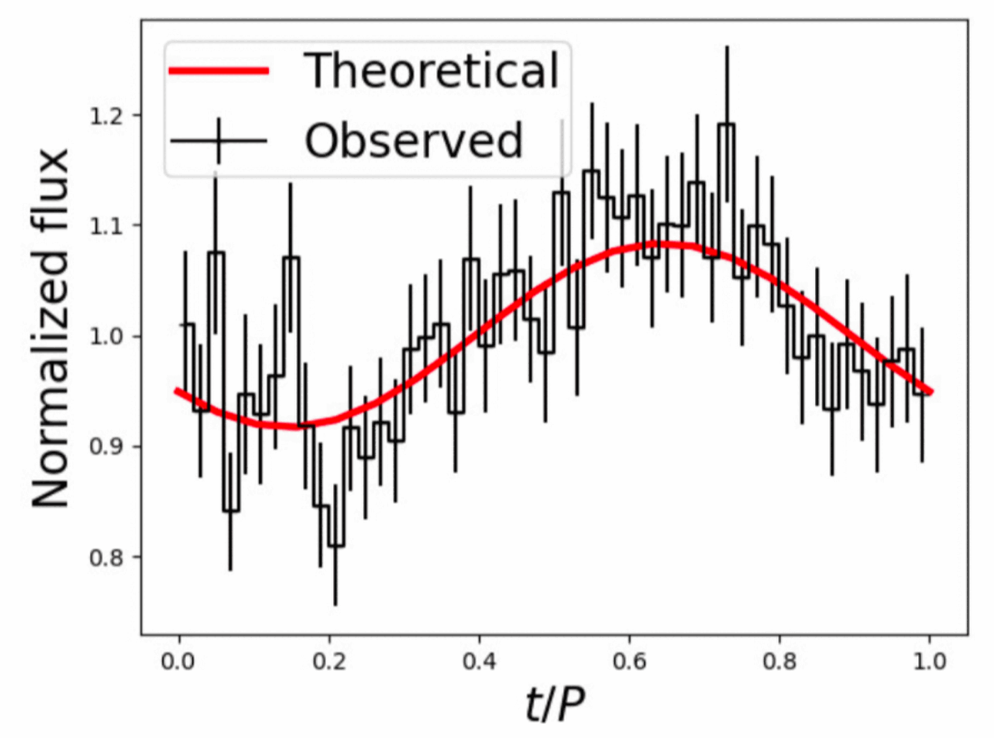
- In X-ray binaries, matter falls along the field lines and forms columns above the poles: the emission comes out sideways (fan beam).
- Exact ray tracing in Schwarzschild, tabulated, including for points above the surface; Doppler included.
- Genetic algorithm for the priors, then MCMC.
1.53+0.52−0.40
M☉
12.1+1.1−0.9
km
Silva, de Lima, Coelho & de Araújo · submitted to JHEAp (2026) · the model
Inside the column, through the spectrum
- The same star as on the previous slide, now through its spectrum: NuSTAR, 3–44 keV, L ≈ 3.7×10³⁶ erg/s — 16 times below the critical luminosity.
- Becker & Wolff (2022) model: a conical column; photons gain energy from the hot electrons and from the infalling gas (thermal and bulk Comptonization) and escape through the walls.
- 12 parameters, 4 independent MCMC chains of 256 walkers. The posterior has two modes; the dominant one wins by Δln 𝒫 ≈ 55.
Silva, de Lima, Coelho & de Araújo · submitted to JHEAp (2026) · the companion
A Be star: a disc at the equator
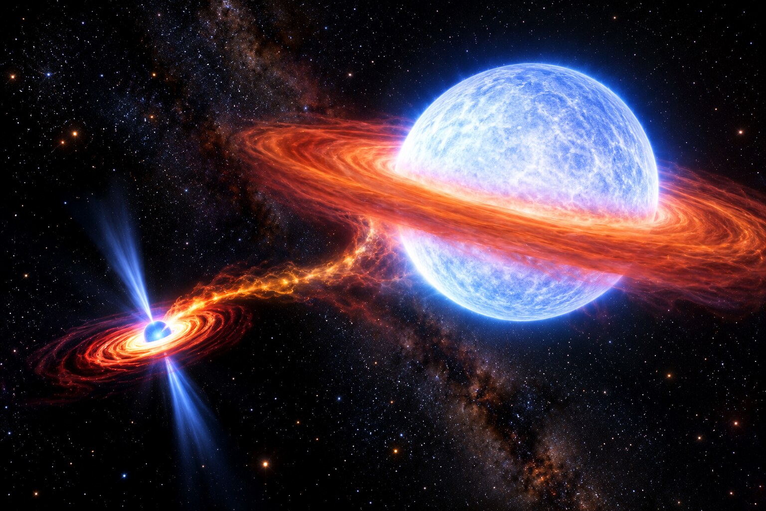
AI-generated illustration- Be stars: hot, of type B and late O, spinning close to break-up and losing gas from the equator, which forms a disc.
- The “e” in O9.7–B0 IIIe stands for the hydrogen emission lines, such as Hα, which come from the disc; a double-peaked profile shows it rotates.
- In 1A 0535+262 the companion is the neutron star, on a 111-day orbit that crosses the edge of the disc — the next slide.
Silva, de Lima, Coelho & de Araújo · submitted to JHEAp (2026) · the system
Where the column’s gas comes from
- 1A 0535+262: a neutron star pulsing every 103 s, with B ≈ 5×10¹² G, on an eccentric orbit — e ≈ 0.45, 111 days — around HD 245770, a Be star (O9.7–B0 IIIe), at 1.8 kpc.
- The Be star spins fast and sheds a disc of gas from its equator.
- At periastron the neutron star crosses the edge of the disc and steals gas: an X-ray outburst every orbit.
- Close to it, the field cuts the disc at the magnetospheric radius and leads the gas to the poles: the columns.
In 2020 a giant outburst reached 1.2×10³⁸ erg/s; in quiescence, ~7×10³⁴ erg/s. The orbit has the system’s eccentricity and period; the stars, the disc and the close-up are schematic.
Silva, de Lima, Coelho & de Araújo · submitted to JHEAp (2026) · the Becker & Wolff model
One equation for the photons in the column
advection
the infalling gas carries the photons along, with the v(y) of the previous slide
bulk Comptonization
the flow converges: scattering off the infalling gas, photons gain energy
diffusion
photons move along the column, with the strong-field cross section σ∥
thermal Comptonization
the Kompaneets term: electrons at Te drive the spectrum towards ~kTe
escape
photons leave through the walls in a time tesc: the fan beam
sources
seed photons: bremsstrahlung, cyclotron and blackbody from the base
How it is solved
Separation of variables: eigenfunctions gn(τ) in optical depth and Whittaker functions in energy. The spectrum is this Green’s function convolved with the sources, adding the wall and the top of the column. Magnetic cross sections with vacuum polarization; cyclotron and iron lines, empirical. The implementation was checked equation by equation.
What the MCMC samples: 12 parameters
Fixed: M = 1.4 M☉, R★ = 10 km, NH and the cyclotron line, outside the band. B has a prior from the line (46.3 keV). The likelihood is Gaussian, with the systematic term fsys, and charges the energy budget Lacc = GMṀ/R★ within a factor of 2.
Silva, de Lima, Coelho & de Araújo · submitted to JHEAp (2026) · results
A hot, tall column — and a missing piece
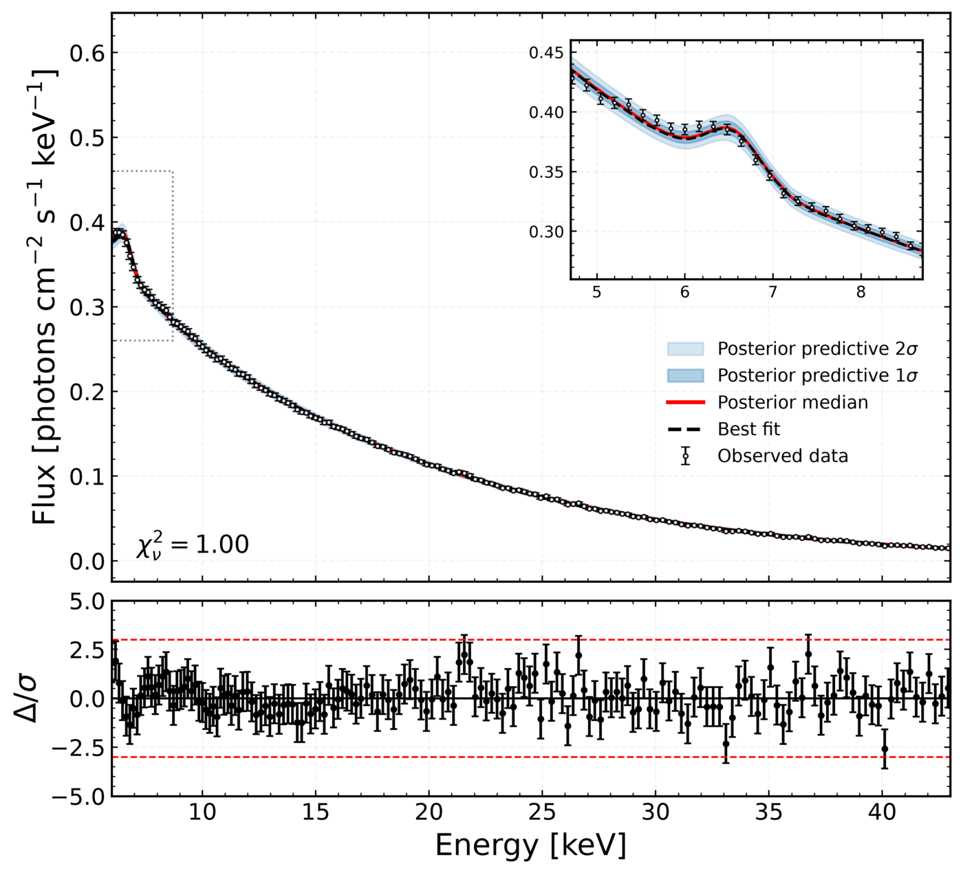
8.56×10⁷ K
electron temperature, to 1% · kT ≈ 7.4 keV
4.5 R★
top of the column, ~35 km above the surface
0.070
ψ, bulk/thermal: thermal Comptonization dominates
log θ0 − 1.36 log Ṁ
= −22.32 ± 0.10
the spectrum fixes the combination: more Ṁ, a wider column
A missing piece
The field comes out 2.3σ above that of the cyclotron line — which would then sit at 55 keV, not the measured 46 — and the residuals move together (runs test: z = −3.7). Candidate: recombination between excited Landau levels, seen in this source and absent from the model.
Dominant posterior mode. χ²ν = 1.00 with a free systematic uncertainty is not a goodness-of-fit test: the residuals are the diagnostic.
Brans & Dicke 1961 · Damour & Esposito-Farèse 1993
What if gravity is not Einstein’s?

Cfbolner (Wikimedia Commons) · CC BY-SA 4.0
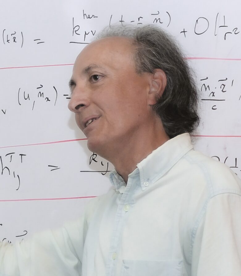
Melirius (Wikimedia Commons) · CC BY 3.0What “coupling to matter” means
Matter measures distances and times with g̃: its rulers and clocks change with φ. Light does not notice — a conformal change leaves null geodesics alone — but the radius matter measures is R = AsRE.
Matter sources the field, □φ = −4πGαT, and feels an extra force, ∝ α∇φ: between two bodies, Geff = G(1 + α²).
In scalar-tensor theories, besides the metric there is a scalar field φ that couples to matter. In the Solar System the coupling is tiny (α² < 10⁻⁵, from the Cassini probe); in a neutron star spontaneous scalarisation can occur: with A = eβφ²/2 and β ≲ −4.35, φ = 0 becomes unstable and the field grows on its own, like spontaneous magnetisation.
Outside the star, the metric is no longer Schwarzschild: it is the Just metric, with a scalar charge Q:
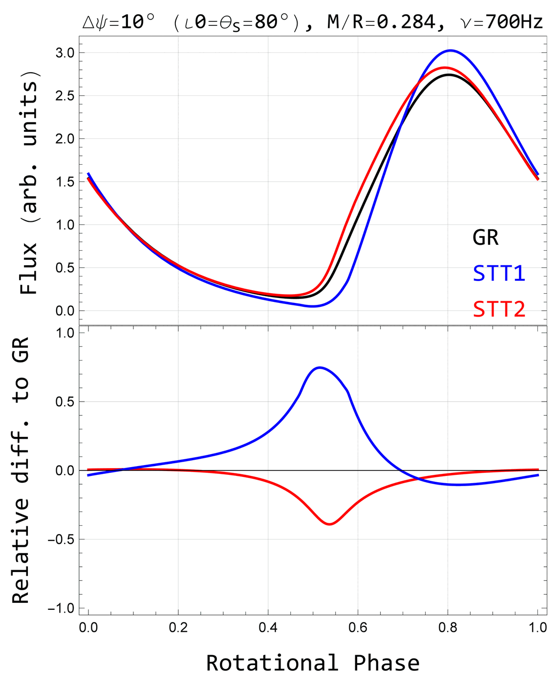
Two stars with the same mass and the same radius — “doppelgängers” — bend light in different ways. The light curve can tell the theories apart.
Ottoni, Coelho, de Lima, Pereira & Rueda · EPJC 84, 1337 (2024)
The same star, different gravity
Ottoni et al. · EPJC 84, 1337 (2024) · results
Up to 80% difference in flux
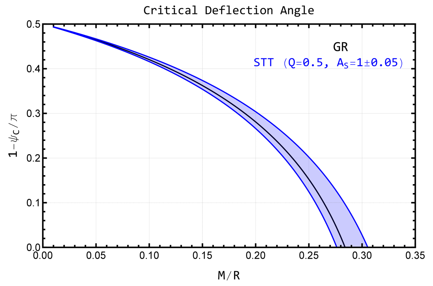

- The compactness at which ψc = π ranges from 0.275 to 0.305 in scalar-tensor theory, against 0.284 in GR.
- The flux from a spot differs from GR by up to ~80%.
- The radius changes by up to ~10% for the same stellar parameters: today, this limits Q ≲ 0.5.
- With NICER, J0740+6620 has C = 0.21–0.28: not yet enough to separate the theories.
Outlook
Radii with smaller uncertainties — eXTP, NewAthena, and gravitational waves from Einstein Telescope and LISA — may constrain scalar-tensor theories through the pulse shape.
Randall & Sundrum 1999 · Shiromizu, Maeda & Sasaki 2000
The Universe on a membrane
In a braneworld, our Universe is a four-dimensional hypersurface — the brane — inside a space with one extra dimension, the bulk. Matter and light are stuck on the brane; only gravity propagates in the bulk.
The idea was put forward to attack the hierarchy problem (why gravity is so weak) and the cosmological-constant problem and accelerated expansion.
- Sμν: local corrections, quadratic in the matter (∝ T²). In a fluid they add ρ²/2λ to the density: they matter when ρ approaches the brane tension λ.
- Eμν: the bulk Weyl tensor projected onto the brane — nonlocal: it cannot be computed from brane quantities alone.
- For λ → ∞ and Eμν → 0, General Relativity is recovered.
In the paper: an effective 4D closure, inspired by the Sahni–Shtanov scenario (2003) — not a complete 5D bulk solution.
The modified TOV equations · SLy equation of state
Same nuclear physics, different gravitation
The equation of state of the matter (SLy) does not change. What changes is how much it gravitates: the star now feels an effective density and pressure.
peff = p + pρλ + ρ²2λ + p𝒰local term (λ) · Weyl sector (𝒰)
dpdr = −(ρ + p) m + 4πr³peffr(r − 2m)matter is conserved: the (ρ + p) factor is the usual one
The local term strengthens attraction and shrinks the star — but only when ρ approaches λ. At the centre of a neutron star ρ ≈ 2×10⁻³ km⁻²; with λ ~ 10⁴ km⁻², ρ/λ ~ 10⁻⁷.
What comes from the bulk
The Weyl sector: screening or extra attraction
Eμν is the imprint of the bulk's gravitational field on the brane. There it acts as an effective fluid — in cosmology, the “dark radiation”. But the brane does not determine this fluid: a closure is needed.
Isotropic closure; the anisotropic Weyl stress (Δ𝒰) is left for future work.
| if… | effect on the star |
|---|---|
| α𝒰 < 0 | ρeff = ρ(1 + α𝒰) < ρ: screening — less mass gravitates, larger and heavier stars |
| α𝒰 > 0 | more attraction: smaller and lighter stars |
| w𝒰 | only appears as w𝒰α𝒰ρ in the effective pressure: it matters little when α𝒰 is small, and it can compensate α𝒰 |
dos Santos Júnior, de Lima & Moraes · arXiv:2607.09836 (2026, submitted) · results
High tension, mildly negative Weyl coupling
Data and inference
GW170817 (radii from the tidal deformability) + NICER: PSR J0740+6620 and PSR J1231−1411 — both of them results of pulse-profile ray tracing. Ensemble MCMC (4 × 32 walkers × 3,000 steps, 288,000 samples), priors centred at large λ and at the GR values.
| median | 68% | GR | |
|---|---|---|---|
| log10(λ/km⁻²) | 3.98 | 2.54 – 5.50 | ∞ |
| α𝒰 | −0.15 | −0.23 – 0.15 | 0 |
| w𝒰 | 0.24 | −0.78 – 0.61 | 0 |
| Mmax (M☉) | 2.30 | 2.22 – 2.44 | 2.05 |
| R1.4 (km) | 13.31 | 12.74 – 13.85 | 11.76 |
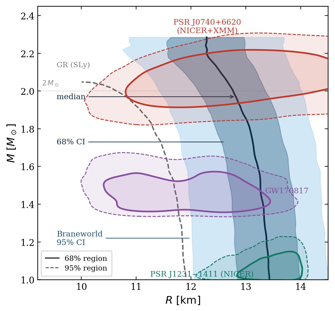
- λ ~ 10⁴ km⁻²: the local term vanishes (ρ/λ ~ 10⁻⁷). The posterior nearly repeats the prior: the data are compatible with high tension, they do not measure λ.
- α𝒰 < 0 in 83% of the samples: a mild screening. It is the Weyl sector, not the local term, that pushes the curve to the right.
- A secondary branch (17%): α𝒰 > 0 and w𝒰 < 0 compensate — smaller R1.4, larger Mmax, compactness near the imposed bound.
- Mmax ≈ 2.3 M☉: consistent with PSR J0952−0607 (2.35 ± 0.11 M☉). GW190814 (2.50–2.67 M☉) only fits in the 95% tail.
- The message: heavier stars are not a generic prediction of braneworlds — they depend on the sign of the Weyl sector.
Itoh 1970 · Bodmer 1971 · Witten 1984 · the strange matter hypothesis
What if iron is not the bottom of the well?
At extreme densities neutrons may dissolve into quarks. The Bodmer–Witten hypothesis goes further: matter made of u, d and s quarks would be the ground state of matter — with an energy per baryon below that of ⁵⁶Fe, 930 MeV.
Pauli: each flavor has its own Fermi sea. A third flavor opens new levels and the top (μ) drops — even after paying for the s mass.
- Nuclei don't decay because that would take ~A simultaneous weak d → s conversions.
- And u–d matter alone must be unstable — otherwise iron itself would have turned into quarks.
- If it holds, “neutron stars” may be quark stars, bound by the strong force.
Alford, Braby, Paris & Reddy 2005 · a QCD-informed equation of state
Dense QCD in three numbers
| a4 = 1 − c | the strong interaction. a4 = 1 means free quarks; perturbative QCD suggests c ≳ 0.3 |
| a2 = ms² − 4Δ² | the s-quark mass against the gap Δ of color superconductivity (CFL phase) — it can be negative |
| B | the bag constant: the cost of opening the QCD vacuum |
At the surface p = 0, but the density is not: ρs ≈ 4B ~ 10¹⁴–10¹⁵ g/cm³. The star is self-bound: at small masses M ∝ R³, unlike a neutron star.
TOV + the tidal equation with the surface jump (Δy = −4πR³ρs/M), solved here. The paper's example gives 2.19 M☉, 11.97 km and Λ = 852 — the panel reproduces it.
Zastrow, Pereira, de Lima & Horvath · PRD 112, 083010 (2025) · the method
Thousands of stars, drawn at random
Each point (a2, a4, B) inside the stability window is a whole family of stars: TOV for M and R, the tidal equation for Λ. The paper drew 263,287 points by Latin hypercube sampling; here the browser draws its own, live.
| accepted range | where it comes from | |
|---|---|---|
| Mmax | 2.13 – 2.33 M☉ | pulsars in binaries (Romani et al. 2022) · GW170817 + GRB 170817A (Rezzolla et al. 2018) |
| R1.4 | 10.00 – 13.25 km | NICER radii — ray tracing — and gravitational waves (compilation by Pang et al. 2023) |
| Λ1.4 | < 970 | tidal deformability from GW170817 |
Amber: the families that pass all three tests. The dashed lines show how far the accepted ones reach — and they converge to the paper's limits.
Zastrow, Pereira, de Lima & Horvath · PRD 112, 083010 (2025) · results
Interacting quarks, a dense surface
| combined constraints | range |
|---|---|
| a4 | 0.18 – 0.81 |
| a2 (10³ MeV²) | −202 – 42 |
| B1/4 (MeV) | 114 – 185 |
| R1.4 (km) | 10.00 – 12.26 |
| Λ1.4 | 270 – 970 |
| ρsurface (10¹⁵ g/cm³) | 0.29 – 0.60 |
| cs/c | 0.51 – 0.85 |
The sound speed exceeds c/√3 ≈ 0.58 — the conformal limit of QCD at infinite density — when a2 < 0.
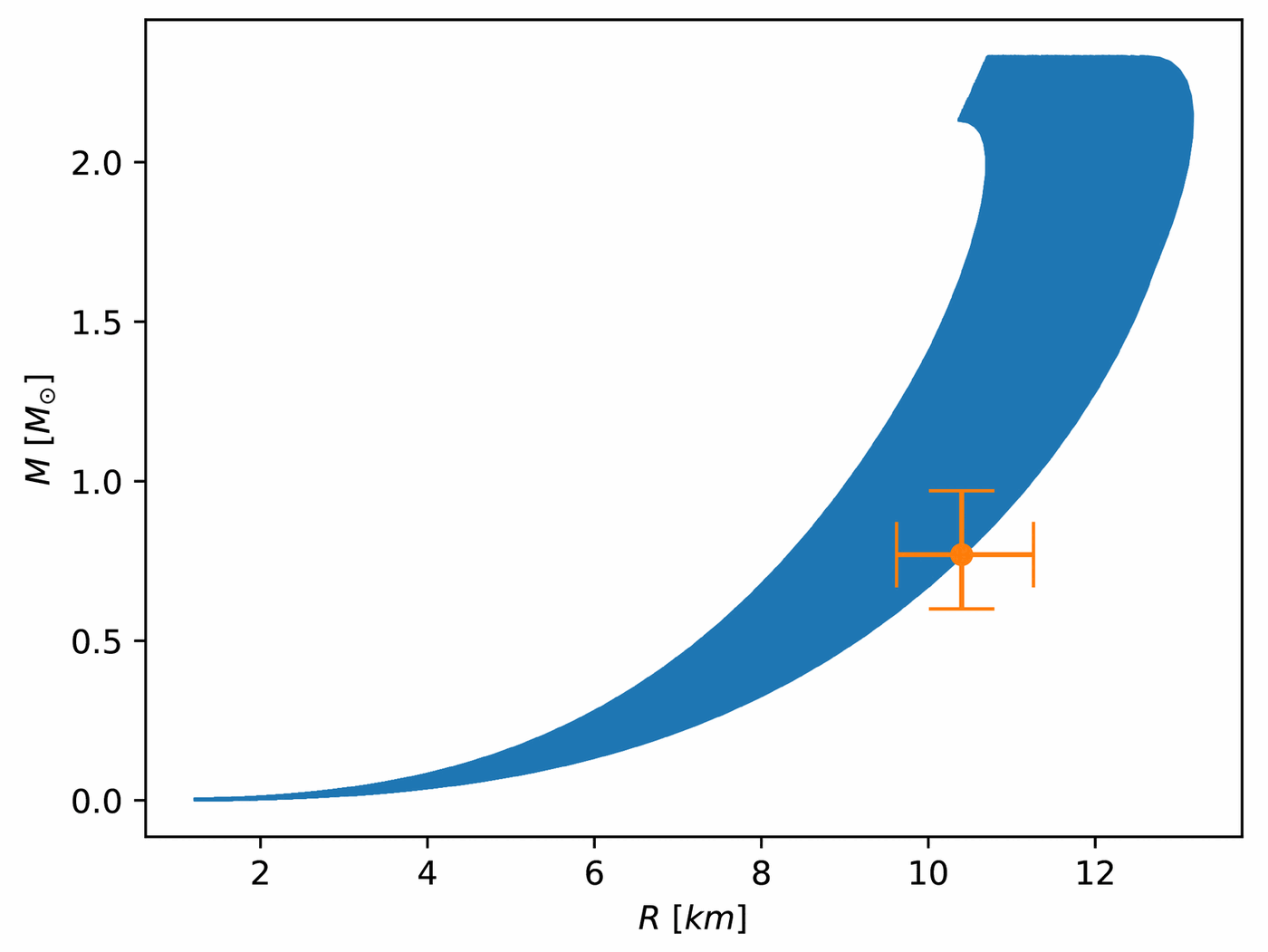
- a4 ≲ 0.81: the matter departs by at least 20% from free quarks. Strong interactions cannot be neglected, at any mass.
- Δ ≲ 230 MeV (with ms = 100 MeV), from the lower limit on a2 — in line with the independent bound of ≲ 216 MeV (Kurkela et al. 2024).
- The surface jumps from vacuum to 1.1–2.2 ρsat: a number that enters the tides, the oscillation modes and the star's mountains.
- R1.4 = 10.0–12.3 km, like a neutron star: the radius alone cannot tell them apart; the tides can.
- XMMU J1732−344 (0.77 M☉, 10.4 km, in HESS J1731−347) falls on the curves effortlessly — a quark-star candidate, if the atmosphere model behind its radius is right.
Pereira, Ottoni, Coelho, Rueda & de Lima · PRD 110, 103014 (2024)
When core and crust do not spin together
Almost every calculation treats a pulsar as a rigid body. But the interior may be superfluid, have a phase transition — a quark core — or gain accreted layers that spin differently, like the Sun's tachocline.
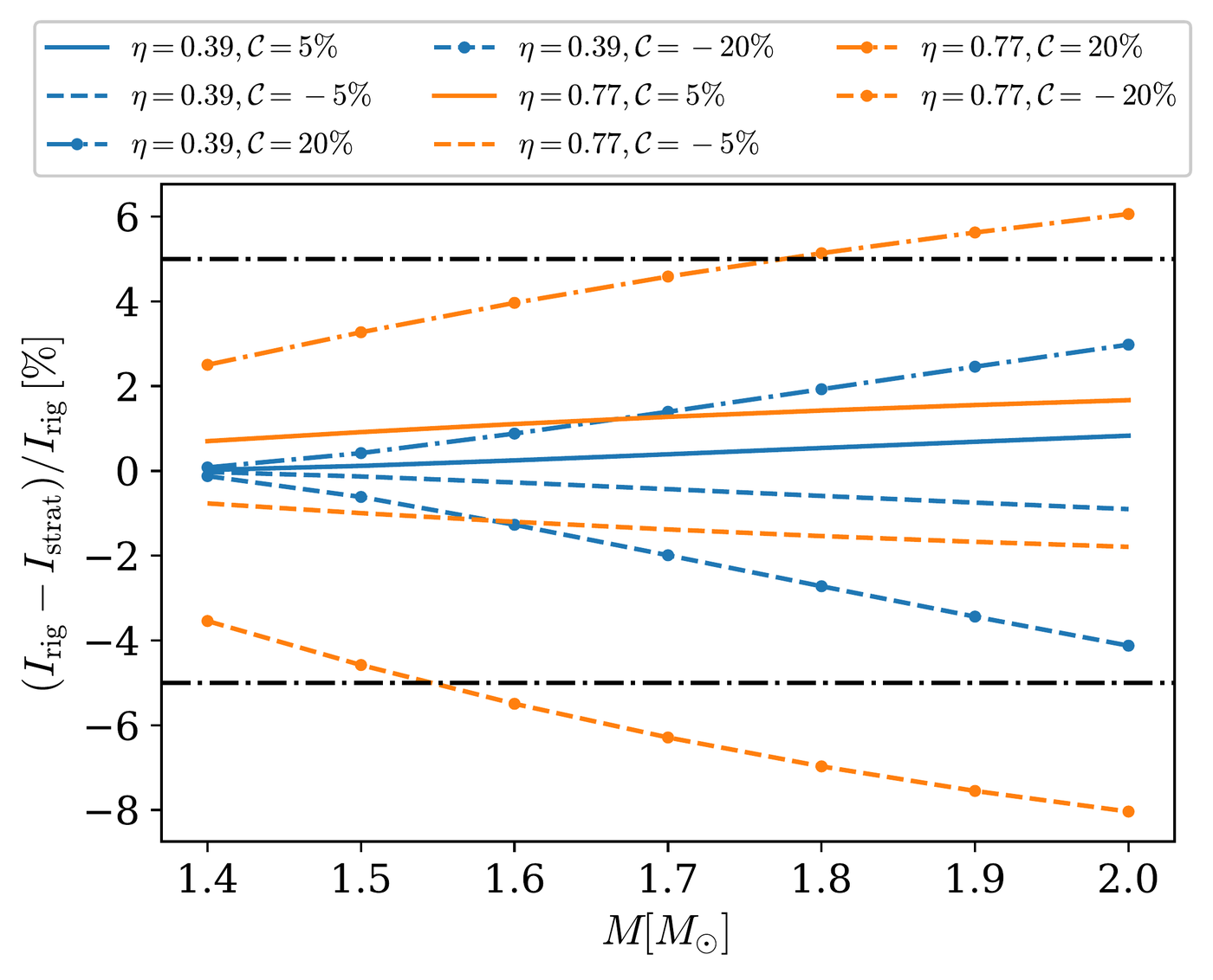
J comes from the derivative of ω̄ at the surface, so it feels the jump: the same star, with the same Ω⁺, has a different moment of inertia.
Pereira, Ottoni, Coelho, Rueda & de Lima · PRD 110, 103014 (2024) · results
Rigid rotation is an assumption — and it has a cost
- Near the surface, ΔI/I → ΔΩ/Ω⁺; below ~40% of the radius the effect vanishes. It grows fast for R★ ≳ 0.6 R, and more in light stars.
- Hybrid stars: the jump sits at the transition to the quark core, and only exceeds 5% with 𝒞 ~ 20% and R★ ≳ 0.8 R (figure).
- In the radius: with a known mass, ΔR/R = ½ ΔI/I. Ten percent in I is 5% in R — the size of the NICER error bars, which come from ray tracing.
- Direct measurement of I: the double pulsar J0737−3039A should give I to 11% by 2030 (today, I45 = 1.15–1.48). Jumps of 10–20% in Ω cannot be told from rigid rotation.
- Energy: with I 10–20% larger, five Fermi gamma-ray pulsars with Lγ > Ė fit back within the rotational energy.
- I-Love-Q: the quadrupole depends on another function besides J — the universal relations weaken. And in CCOs, accreted layers may spin differently for up to ~10 thousand years.
| pulsar (Fermi) | Lγ/Ė, I0 | +10% | +20% |
|---|---|---|---|
| J1057−5851 | 1.19 | > 1 | 0.99 |
| J1522−5735 | 1.09 | 0.99 | 0.91 |
| J1650−4601 | 1.11 | > 1 | 0.92 |
Conclusions
From geometry to observation — and back
- In a neutron star, light bending, redshift and delays are not corrections: they define the image and the light curve.
- Backward ray tracing — with the exact integral when the compactness calls for it — links the metric to what a telescope measures.
- Applied to Chandra, XMM-Newton and NuSTAR data, it gave the mass, radius, field and spot geometry of magnetars and of an accreting star — and, through its spectrum, the temperature and height of its column.
- Since the light curve depends only on the exterior metric, it also tests gravity: scalar-tensor theories and braneworld.
- And the interior matters: quark stars and stratified rotation change the M, R and I that ray tracing measures.
Next steps
- Magnetised atmospheres and exact ray tracing together, for isolated cooling stars.
- Fast rotation and metrics beyond Schwarzschild in the same fits.
- Data from the next generation: eXTP, NewAthena, STROBE-X.
The panels in this seminar run in the browser: rafael-lima.pages.dev/talks.
Image credits
Freely licensed photos and figures
Albert Einstein — Ferdinand Schmutzer / Adam Cuerden · public domain
Karl Schwarzschild — unknown author · public domain
M87* (EHT) — Event Horizon Telescope Collaboration · CC BY 4.0
Sgr A* (EHT) — EHT Collaboration · CC BY 4.0
Jocelyn Bell, 1967 — Roger W Haworth · CC BY-SA 2.0
Antony Hewish — Woodruff T. Sullivan III / NRAO/AUI Archives (NRAO/AUI/NSF) · CC BY 4.0
Chart record of CP 1919, 1967 — Bill Thompson (Billthom) · CC BY-SA 4.0
Neutron star over Manhattan — NASA's Goddard Space Flight Center · public domain
1919 eclipse — ESO/Landessternwarte Heidelberg-Königstuhl/F. W. Dyson, A. S. Eddington, & C. Davidson · CC BY 4.0
SMACS 0723 (JWST) — NASA, ESA, CSA, and STScI · public domain
NICER — NASA · public domain
XMM-Newton — ESA/XMM-Newton · CC BY-SA 3.0 IGO
Chandra — NASA/CXC/NGST · public domain
Pulsar (illustration) — NASA · public domain
Magnetar (illustration) — ESO/L. Calçada · CC BY 4.0
Carl Brans — Cfbolner · CC BY-SA 4.0
Thibault Damour — Melirius · CC BY 3.0
PSR J0030+0451: hot-spot models — NASA's Goddard Space Flight Center · public domain
Paper figures (Part IV) — de Lima et al., ApJ 889, 165 (2020); de Lima et al., JHEAp 42, 52 (2024, CC BY 4.0 on arXiv); Silva et al., Galaxies 11, 18 (2023, CC BY 4.0); Ottoni et al., EPJC 84, 1337 (2024, CC BY 4.0); dos Santos Júnior, de Lima & Moraes, arXiv:2607.09836 (CC0); Pereira et al., PRD 110, 103014 (2024); Zastrow et al., PRD 112, 083010 (2025); Silva, de Lima, Coelho & de Araújo (submitted to JHEAp, 2026)
Simulated Sobral plate — positions from the Tycho-2 catalogue (Høg et al., A&A 355, L27, 2000), via VizieR/CDS
Be/X binary (illustration) — AI-generated
P–Ṗ diagram — ATNF pulsar catalogue 2.8.1 (Manchester et al., AJ 129, 1993, 2005)
Thank you
Questions?
Slides, animations and dashboards available at rafael-lima.pages.dev/talks