UDESC · CCT · Department of Physics

Seminar · 2026

SCARLET · TeV–PeV

Neutrinos, antineutrinos
and inelasticity

Structure-function model dependence of the inelasticity of TeV–PeV neutrino interactions and of neutrino–antineutrino separation in neutrino telescopes

Outline

Four parts

I

IceCube

What the detector measures and how composition enters the analysis

II

DIS

Structure functions and the separation of ν and ν̄

III

GENIE and SCARLET

Models, implementation and constraints from data

IV

Results

Composition shifts, kinematic origin and statistical scale

Main question

Similar means, different compositions

How much does the inferred ν/ν̄ composition change when we change the interaction templates?

The shift depends on both the template difference and the remaining separating power.

I

Part I

IceCube

Light in ice and flux composition without a lepton-charge measurement

John Hardin · CC BY 4.0

The observatory

A cubic kilometre of instrumented ice

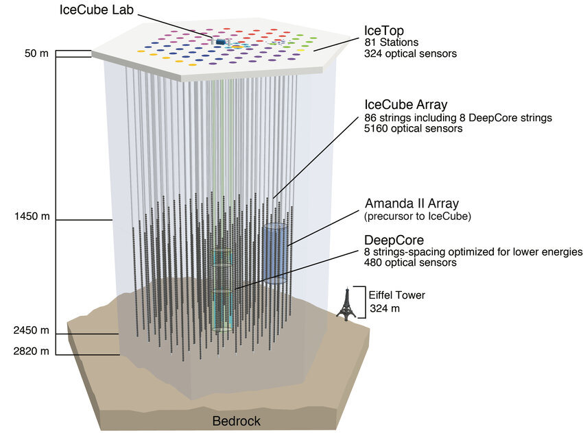
IceCube detector geometry — K. Andeen & M. Plum · IceCube · CC BY 4.0

5,160 optical modules on 86 strings.

Sensors at depths of 1,450–2,450 m.

Charged particles produce Cherenkov light. Signal times and intensities constrain the event geometry and energy.

IceCube · icecube.wisc.edu/science/icecube/

Charged-current interactions

The cascade and muon share the energy

ν_μ + N → μ⁻ + X ν̄_μ + N → μ⁺ + X

The hadronic cascade receives approximately yE_ν. The muon receives (1 − y)E_ν.

The detector measures light and reconstructs energies. The μ⁻/μ⁺ charge is unavailable event by event.

IceCube, Phys. Rev. D 99 (2019) 032004 · arXiv:1808.07629

Visible energy

True and reconstructed inelasticity

Energy partition · example without smearing

y

κ

y = E_had / E_ν

y_vis = κy / [(1 − y) + κy]Simplified response with full containment

κ represents the cascade response. Migration and selection enter the forward fit.

The motivating measurement

IceCube already uses inelasticity

5

years of contained events

1–100 TeV

approximate inelasticity measurement range

0.77

flux ratio relative to HKKMS, with +0.44/−0.25

Sensitivity to the atmospheric ratio comes from 770 GeV–21 TeV.

IceCube · arXiv:1808.07629

Three distinct quantities

Interaction fraction, event fraction and flux ratio

Quantity	Definition	Ingredients
f	ν̄ fraction of CC interactions	True distributions at fixed energy
f_ev	ν̄ fraction of selected events	Fluxes, cross sections and response
r	Scale on HKKMS Φ_νμ/Φ_ν̄μ	Joint fit with flux nuisances

A shift in f does not translate directly into the same shift in r.

II

Part II

DIS

Structure functions determine the distributions that separate ν and ν̄

Kinematics

The domain of Bjorken x and Q²

Q² = 2M E_ν xy W² = M² + Q²(1/x − 1)

x measures the nucleon momentum fraction sampled by the interaction. Q² sets the resolution scale.

(M_W² / [Q² + M_W²])²The propagator suppresses Q² far above M_W²

Manuscript · §2

CC cross section

F₂, F_L and xF₃

d²σ^ν,ν̄/dxdy = (G_F²ME/π) (M_W²/[Q²+M_W²])²

× [F₂(1−y+y²/2) − F_Ly²/2 ± xF₃ y(1−y/2)]

The xF₃ term changes sign between ν and ν̄. Positive F_L suppresses the high-y tail.

Expression without lepton-mass and target-mass terms. The calculation uses each configuration’s prescriptions.

Manuscript · eq. (2.1)

Analytic illustration

Helicity and the y distribution

LO · F_L = 0 · no scaling violations

R = ±xF₃/F₂

dσ/dy ∝ 1 − y + y²/2
+ R(y − y²/2)

⟨y⟩ = (7 + 5R)/(16 + 8R)

R = +1: a flat distribution.
R = −1: a distribution proportional to (1 − y)².

Manuscript · eqs. (2.2)–(2.3)

Mixtures

Composition depends on the templates

Actual Tier 1 distributions on water

Energy (index)

Antineutrino fraction f

p(y) = (1 − f)p_ν(y) + fp_ν̄(y)

The two distributions approach each other as energy increases. The same change in f then produces a smaller shape change.

Paper data · WP-F · 100 bins em y

Bias mechanism

Separation enters the denominator

δf ≃ − [(1−f)δ_ν + fδ_ν̄] / [⟨y⟩_ν − ⟨y⟩_ν̄]

δ_ν and δ_ν̄ are the true mean shifts relative to the template means.

As separation decreases, a small shape mismatch can shift the composition substantially. The full fit uses the entire distribution.

Manuscript · eq. (2.4)

Dipole description

The boson fluctuates into a quark pair

F_T,L = Q²/(4π²) Σ_q₁q̄₂ ∫ d²r ∫ dz D_T,L^V(z,r) σ_qq̄(x̃,r)

Current wave functions determine the coupling to the pair. The dipole cross section describes its interaction with the target.

BGK includes DGLAP evolution of the gluon. This work uses a HERA fit and three matching prescriptions.

BGK, Phys. Rev. D 66 (2002) 014001 · Manuscript §3

Sea matching

A window between two descriptions

Blend weight w(x)

S = wD + (1 − w)C
w = 1 − t²(3 − 2t)
t = ln(x/0.01)/ln(10)

Below x = 0.01, the dipole part. Above x = 0.1, the conventional description.

Tier 1 preserves the dipole shape inside the window. Tier 2 tests the blend and conventional shape.

Manuscript · eqs. (3.2)–(3.3)

III

Part III

GENIE and SCARLET

A common implementation for structure functions and inference

Architecture

The roles of GENIE and SCARLET

Layer	Role
GENIE R-3_06_02	Channels, kinematics and event-generation infrastructure
SCARLET · scarlet_physics	Wave functions, dipoles and structure functions
SCARLET · scarlet_genie	Adapters for the GENIE DIS and charm algorithms
SCARLET · analysis	Integration, templates, controls and composition fits

GENIE remains a dependency. The adapters replace algorithms through configuration.

SCARLET · src/genie_interface · Manuscript §3

Configurations

One reference and three dipoles

Model	Construction	Status
HEDIS / NLO	HERAPDF1.5 + APFEL	External reference
Tier 1	BGK + valence subtraction + dipole shape	Admitted by the relative criterion
Tier 2	Same BGK, blend and conventional shape	Variations failing the pull condition
Bodek–Yang	GENIE conventional structure functions	Separate comparison

“Family” includes NLO and the three dipoles. Bodek–Yang is separate.

Manuscript · §§3–4

Reach of the data

Data constrain other scales

Data set	x	Q² (GeV²)	Role
HERA	≤ 0.01	≤ 650	Dipole fit
NuTeV	0.015, 0.045, 0.08	1–48	Candidate discrimination
TeV–PeV predictions	Multiple regions	~10²–10⁴	Evolution and matching

The prediction requires extrapolating the fitted inputs. The study quantifies differences between those prescriptions.

Manuscript · §4, Reach of these constraints

Selection and history

Tier 1 passes by a narrow margin

NuTeV	χ²/N (x ≤ 0.1 / all x)	Largest pull
Bodek–Yang	2.18 / 2.29	−5.5σ
Tier 1	1.67 / 1.68	−2.77σ
Tier 1 without 1.032	—	−4.1σ
Tier 1 without radiation	—	−4.3σ

The criterion was revised with results already known. The factor 1.032 entered with that revision.

Manuscript · Table 1 · Histórico em apêndice / history in appendix

NLO reference

HEDIS remains an external reference

HEDIS variant	NuTeV χ²/N	CCFR χ²/N
Nominal	2.54 / 2.87	5.23 / 3.85
× 1.032	2.72 / 3.06	5.23 / 3.85
Iron factor	2.90 / 3.00	2.43 / 2.29
Iron × 1.032	3.09 / 3.20	2.43 / 2.29

The nuclear factor improves CCFR and worsens NuTeV. Every variant fails the NuTeV criterion.

Manuscript · Table 1

Charm treatment

An inverted propagator in G18

G_W² ∝ (1 + Q²/M_W²)²Form found in AivazisCharmPXSecLO

G_W² ∝ (1 + Q²/M_W²)⁻²Correct propagator dependence

The cross-section effect is ≤ 0.4% up to 1 TeV, but grows when extrapolating G18. HEDIS does not use this model.

The comparisons use charm consistent with each configuration’s structure functions.

GENIE issue #558 · Manuscript §3 and appendix C

IV

Part IV

Results

Similar shapes, loss of separation and composition shifts

Distribution in x and Q²

The kinematic domain changes with energy

Tier 1, ν_μ, water. Cross-section fraction per 0.25 × 0.25 decade cell.

x < 0.01: from 3.1% to 55% between 1 TeV and 1 PeV.

The occupancy map does not isolate saturation effects.

Paper WP-F outputs

Energy

Paper data · WP-F · Table 2

Separating power

Δ⟨y⟩ falls from 0.12 to 0.008

The ν–ν̄ separation decreases far more than the spread of model means.

Within the family, the means differ by at most about 0.005.

Solid lines: ν.
Dashed lines: ν̄.

Integrated means on water

Manuscript · Figure 2 · dados WP-F

Shape fits

Small differences shift the fraction

Templates of A fitted to the expected mixture of B.

Maximum over ordered pairs and f = 0.15–0.50, with 20 bins in y.

The physical fit uses 0 ≤ f ≤ 1. Large high-energy shifts accompany a loss of information.

Maximum |δf| · physical domain

Manuscript · Table 3 · Figure 3

Identifiability

A large bias can occur without a poor fit

2.4

σ_f√N at 1 TeV

31

σ_f√N at 1 PeV

≤ 1.2

deviance for 18 degrees of freedom at exposure N_bias

At the exposure where |δf| equals the statistical error, goodness of fit may not reveal the shift.

Manuscript · §5 e Table 3

Implementation controls

Common targets and cuts

E (TeV)	Nominal	Free nucleons	+ W > 2 GeV	+ Q² > 1 GeV²
1	0.026	0.021	0.030	0.023
3	0.026	0.019	0.021	0.017
100	0.065	0.049	0.049	0.048
1000	0.438	0.318	0.318	0.317

Maximum |δf|, Tier 1–NLO. Cuts matter at low energy. Nuclear treatment explains part of the high-energy difference.

Manuscript · Table 4 · physical fits

Regional decomposition

Contributions in x can cancel

Fixed comparison: NLO templates fitted to a Tier 1 mixture with f = 0.25.

Up to 30 TeV: |δf| ≤ 0.019 with cancellations.

Matching dominates at 100 TeV. x < 0.01 dominates from 300 TeV.

One-region-at-a-time replacement

Energy

Manuscript · Table 5 · controlled replacement

Observational comparison

The current measurement does not distinguish the models

All predictions lie within 0.6 times the IceCube 68% half-interval.

Differences from the reference: ≤ 0.004 within the family and ≤ 0.011 for Bodek–Yang.

The chart shows the five visible-energy bins.

True ⟨y⟩ inferred through forward folding

IceCube · arXiv:1808.07629 · Manuscript Table 6

Comparison validation

The forward fit preserves the result

Test	Result
5 models, 11 responses, Asimov	FF − E1 = −0.003 … +0.004
Change in model differences	≤ 0.0006
300 pseudo-experiments per model, bins 1–4	Bias ≤ 0.001
Open bin, ~8 events	Bias up to 0.014; ~50% at boundaries

The real IceCube response remains outside this test.

Manuscript §6 and appendix D.2 · VALIDATION §5f.1

Detector level

The fit includes flux and response

N_i,c(b) = ∫ dE dcosθ dy Φ_i,c P_i (dσ_i/dy) A_i M_i

Atmospheric and astrophysical fluxes, veto, Earth absorption, energy resolution and track selection.

Acceptance was calibrated to IceCube counts after a first Asimov run had already shown the biases.

Calibration changes the shifts by less than 0.01 in r.

Manuscript · §7 · simplified response

Flux ratio

Shifts of 8% and up to 18%

Truth ← templates	δr	Shape part
NLO ← Tier 1	−0.056	−0.025
Tier 1 ← NLO	+0.065	+0.030
NLO ← Tier 2 conv.	−0.107	−0.081
Tier 2 conv. ← NLO	+0.139	+0.103
NLO ← Bodek–Yang	+0.033	+0.091

Asimov, r = 0.77. Tier 1–NLO: roughly half from shapes and half from cross sections and absorption.

Manuscript · Table 7 · complete configurations

Statistical scale

Exposure makes the difference relevant

r = 0.77^+0.32_−0.21Asimov profile at ×1, reference as truth

The error is asymmetric. The comparison uses the biased fit half-interval towards the true value.

×10 keeps the same response. It is not a specific Gen2 forecast.

|δr| / profile half-interval

Exposure

Manuscript · §7, Comparison scale · interval ΔlnL = 1/2

Fit validation

Closure and coverage have distinct scopes

Diagnostic	×1	×10
Estimator r̂	Upward bias of 6–10%	Diagnostics in ρ = ln r
Closure in ρ	Fails; \|bias\| ≤ 0.035	0 failures in 65 tests
Profile coverage	Not evaluated	68.30 ± 0.23% / 95.01 ± 0.11%

ρ = ln r was adopted after the failure. The transformation preserves the maximum and maps the interval.

Manuscript · §7.4 and appendix D.1

Interpretation limits

What the results establish

1

Differences between prescriptions

The family is finite and shares inputs. Its envelope has no probabilistic coverage.

2

Complete configurations in the detector

Nuclear and normalisation effects have not been separated at this level.

3

Inference in a proxy

The tests do not establish a bias in IceCube’s measurement or validate its real response.

Conclusions

Composition inference requires testing the distributions

Similar means do not guarantee stable inferred composition.

0.12 → 0.008

decrease in ν–ν̄ separation

8–18%

r shifts within the family, in the proxy

0.8–1.6

times the profile error at ×10

SCARLET · Manuscript em preparação / manuscript in preparation · 30 Oct 2026

Sources and credits

References and data

This work
R. C. R. de Lima and B. D. S. Moreira
Structure-function model dependence of the inelasticity of TeV–PeV neutrino interactions and of neutrino–antineutrino separation in neutrino telescopes
Manuscript in preparation, 30 October 2026 version.

IceCube
Phys. Rev. D 99 (2019) 032004
arXiv:1808.07629
icecube.wisc.edu/science/icecube

Models
CSMS: JHEP 08 (2011) 042
BGK: Phys. Rev. D 66 (2002) 014001
GENIE and HEDIS: manuscript references.

Images and numbers
IceCube Lab: John Hardin, CC BY 4.0.
Detector: K. Andeen and M. Plum, CC BY 4.0.
Study charts: SCARLET outputs, provenance in assets/data-sources.json.

SCARLET · TeV–PeV

Questions?

Inelasticity, composition and structure-function dependence

Neutrinos, antineutrinosand inelasticity

IceCube

DIS

GENIE and SCARLET

Results

IceCube

DIS

GENIE and SCARLET

Results

Differences between prescriptions

Complete configurations in the detector

Inference in a proxy

Questions?

Notes

Neutrinos, antineutrinos
and inelasticity